What Did We Learn?

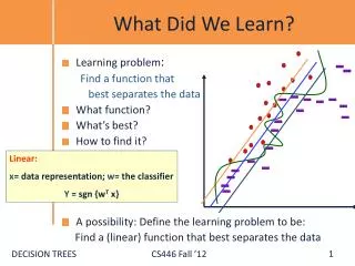
1. What Did We Learn? • Learning problem: Find a function that best separates the data • What function? • What’s best? • How to find it? • A possibility: Define the learning problem to be: Find a (linear) function that best separates the data Linear: x= data representation; w= the classifier Y = sgn {wT x}

2. Introduction - Summary • We introduced the technical part of the class by giving two examples for (very different) approaches to linear discrimination. • There are many other solutions. • Question 1: Our solution assumed that the target functions are linear. Can we learn a function that is more flexible in terms of what it does with the feature space? • Question 2: Can we say something about the quality of what we learn (sample complexity, time complexity; quality)

3. x2 x Decision Trees • We decoupled the generation of the feature space from the learning. • Argued that we can map the given examples into another space, in which the target functions are linearly separable. • Do we always want to do it? • How do we determine what are good mappings? • The study of decision trees may shed some light on this. • Learning is done directly from the given data representation. • The algorithm ``transforms” the data itself. Think about the Badges problem What’s the best learning algorithm?

4. Decision Trees • A hierarchical data structure that represents data by implementing a divide and conquer strategy • Can be used as a non-parametric classification and regression method • Given a collection of examples, learn a decision tree that represents it. • Use this representation to classify new examples B A C

5. Color Blue red Green Shape Shape B triangle circle circle square square B A B C A The Representation • Decision Trees are classifiers for instances represented as feature vectors (color= ; shape= ; label= ) • Nodes are tests for feature values • There is one branch for each value of the feature • Leaves specify the category (labels) • Can categorize instances into multiple disjoint categories (color= RED ;shape=triangle) Decision Trees Evaluation of a Decision Tree Learning a Decision Tree

6. Blue red Green Boolean Decision Trees • As Boolean functions they can represent any Boolean function. • Can be rewritten as rules in Disjunctive Normal Form (DNF) • Green^square positive • Blue^circle  positive • Blue^square  positive • The disjunction of these rules is equivalent to the Decision Tree • What did we show? Color Decision Trees Shape Shape + triangle circle circle square square + - - + +

7. X<3 no yes Y>7 Y<5 no yes yes no X < 1 + - - + + - Decision Boundaries • Usually, instances are represented as attribute-value pairs (color=blue, shape = square, +) • Numerical values can be used either by discretizing or by using thresholds for splitting nodes • In this case, the tree divides the features space into axis-parallel rectangles, each labeled with one of the labels Y + + + Decision Trees 7 + + - 5 + - - 1 3 X

8. Color Blue red Green Shape Shape + triangle circle circle square square + - - + + Decision Trees • Output is a discrete category. Real valued outputs are possible (regression trees) • There are efficient algorithms for processing large amounts of data (but not too many features) • There are methods for handling noisy data (classification noise and attribute noise) and for handling missing attribute values Decision Trees

9. Outlook Rain Sunny Overcast Humidity Wind High Normal Strong Weak Yes Yes No No Yes Decision Trees • Can represent any Boolean Function • Can be viewed as a way to compactly represent a lot of data. • Advantage: non-metric data • Natural representation: (20 questions) • The evaluation of the Decision Tree Classifier is easy • Clearly, given data, there are many ways to represent it as a decision tree. • Learning a goodrepresentation from data is the challenge.

10. Representing Data • Think about a large table, N attributes, and assume you want to know something about the people represented as entries in this table. • E.g. own an expensive car or not; • Simplest way: Histogram on the first attribute – own • Then, histogram on first and second (own & gender) • But, what if the # of attributes is larger: N=16 • How large are the 1-d histograms (contingency tables) ? 16 numbers • How large are the 2-d histograms? 16-choose-2 = 120 numbers • How many 3-d tables? 560 numbers • With 100 attributes, the 3-d tables need 161,700 numbers • We need to figure out a way to represent data in a better way, and figure out what are the important attributes to look at first. • Information theory has something to say about it – we will use it to better represent the data. Representation

11. Day Outlook Temperature Humidity WindPlay Tennis 1 Sunny Hot High Weak No 2 Sunny Hot High Strong No 3 Overcast Hot High Weak Yes Outlook 4 Rain Mild High Weak Yes 5 Rain Cool Normal Weak Yes 6 Rain Cool Normal Strong No Rain Sunny Overcast 7 Overcast Cool Normal Strong Yes Humidity Wind 8 Sunny Mild High Weak No 9 Sunny Cool Normal Weak Yes High Normal Strong Weak Yes Yes No 10 Rain Mild Normal Weak Yes No 11 Sunny Mild Normal Strong Yes 12 Overcast Mild High Strong Yes 13 Overcast Hot Normal Weak Yes 14 Rain Mild High Strong No Basic Decision Trees Learning Algorithm Yes Data is processed in Batch (i.e. all the data available) Recursively build a decision tree top down.

12. Basic Decision Tree Algorithm • Let S be theset of Examples • Label is the target attribute (the prediction) • Attributes is the set of measured attributes • Create a Root node for tree If all examples are labeled the same return a single node tree with Label OtherwiseBegin A = attribute in Attributes that best classifies S for each possible value v of A Add a new tree branch corresponding to A=v Let Svbe the subset of examples in S with A=v if Sv is empty: add leaf node with the common value of Label in S Else: below this branch add the subtree ID3(Sv, Attributes - {a}, Label) End Return Root ID3

13. Picking the Root Attribute • The goal is to have the resulting decision tree as small as possible (Occam’s Razor) • Finding the minimal decision tree consistent with the data is NP-hard • The recursive algorithm is a greedy heuristic search for a simple tree, but cannot guarantee optimality. • The main decision in the algorithm is the selection of the next attribute to condition on.

14. A 1 0 B 1 0 - + - A 1 0 - + Picking the Root Attribute • Consider data with two Boolean attributes (A,B). < (A=0,B=0), - >: 50 examples < (A=0,B=1), - >: 50 examples < (A=1,B=0), - >: 0 examples < (A=1,B=1), + >: 100 examples What should be the first attribute we select? Splitting on A: we get purely labeled nodes. Splitting on B: we don’t get purely labeled nodes. What if we have: <(A=1,B=0), - >: 3 examples

15. A B 1 1 0 0 100 53 - - B A 1 1 0 0 100 50 3 100 - - + + Picking the Root Attribute • Consider data with two Boolean attributes (A,B). < (A=0,B=0), - >: 50 examples < (A=0,B=1), - >: 50 examples < (A=1,B=0), - >: 0 examples 3 examples < (A=1,B=1), + >: 100 examples Trees looks structurally similar; which attribute should we choose? Advantage A. But… Need a way to quantify things

16. Picking the Root Attribute • The goal is to have the resulting decision tree as small as possible (Occam’s Razor) • The main decision in the algorithm is the selection of the next attribute to condition on. • We want attributes that split the examples to sets that are relatively pure in one label; this way we are closer to a leaf node. • The most popular heuristics is based on information gain, orginated with the ID3 system of Quinlan.

17. In general, when pi is the fraction of examples labeled i: Entropy • Entropy (impurity, disorder) of a set of examples, S, relative to a binary classification is: where is the proportion of positive examples in S and is the proportion of negatives. If all the examples belong to the same category: Entropy = 0 If all the examples are equally mixed (0.5, 0.5): Entropy = 1 Entropy can be viewed as the number of bits required, on average, to encode the class of labels. If the probability for + is 0.5, a single bit is required for each example; if it is 0.8 -- can use less then 1 bit.

18. 1 1 1 -- -- -- + + + Entropy • Entropy (impurity, disorder) of a set of examples, S, relative to a binary classification is: where is the proportion of positive examples in S and is the proportion of negatives. If all the examples belong to the same category: Entropy = 0 If all the examples are equally mixed (0.5, 0.5): Entropy = 1

19. 1 1 1 Entropy High Entropy – High level of Uncertainty Low Entropy – No Uncertainty. • Entropy (impurity, disorder) of a set of examples, S, relative to a binary classification is: where is the proportion of positive examples in S and is the proportion of negatives. If all the examples belong to the same category: Entropy = 0 If all the examples are equally mixed (0.5, 0.5): Entropy = 1

20. Outlook Sunny Overcast Rain Information Gain • The information gain of an attribute a is the expected reduction in entropy caused by partitioning on this attribute where is the subset of S for which attribute a has value v and the entropy of partitioning the data is calculated by weighing the entropy of each partition by its size relative to the original set • Partitions of low entropy (imbalanced splits) lead to high gain • Go back to check which of the A, B splits is better

21. Day Outlook Temperature Humidity WindPlay Tennis 1 Sunny Hot High Weak No 2 Sunny Hot High Strong No 3 Overcast Hot High Weak Yes 4 Rain Mild High Weak Yes 5 Rain Cool Normal Weak Yes 6 Rain Cool Normal Strong No 7 Overcast Cool Normal Strong Yes 8 Sunny Mild High Weak No 9 Sunny Cool Normal Weak Yes 10 Rain Mild Normal Weak Yes 11 Sunny Mild Normal Strong Yes 12 Overcast Mild High Strong Yes 13 Overcast Hot Normal Weak Yes 14 Rain Mild High Strong No An Illustrative Example

22. Day Outlook Temperature Humidity WindPlay Tennis 1 Sunny Hot High Weak No 2 Sunny Hot High Strong No 3 Overcast Hot High Weak Yes 4 Rain Mild High Weak Yes 5 Rain Cool Normal Weak Yes 6 Rain Cool Normal Strong No 7 Overcast Cool Normal Strong Yes 8 Sunny Mild High Weak No 9 Sunny Cool Normal Weak Yes 10 Rain Mild Normal Weak Yes 11 Sunny Mild Normal Strong Yes 12 Overcast Mild High Strong Yes 13 Overcast Hot Normal Weak Yes 14 Rain Mild High Strong No An Illustrative Example (II) 9+,5-

23. Humidity WindPlay Tennis High Weak No High Strong No High Weak Yes High Weak Yes Normal Weak Yes Normal Strong No Normal Strong Yes High Weak No Normal Weak Yes Normal Weak Yes Normal Strong Yes High Strong Yes Normal Weak Yes High Strong No An Illustrative Example (II) 9+,5- E=.94

24. Humidity WindPlay Tennis High Weak No High Strong No High Weak Yes High Weak Yes Normal Weak Yes Normal Strong No Normal Strong Yes High Weak No Normal Weak Yes Normal Weak Yes Normal Strong Yes High Strong Yes Normal Weak Yes High Strong No An Illustrative Example (II) Humidity High Normal 9+,5- 3+,4- E=.94 6+,1- E=.985 E=.592

25. Humidity WindPlay Tennis High Weak No High Strong No High Weak Yes High Weak Yes Normal Weak Yes Normal Strong No Normal Strong Yes High Weak No Normal Weak Yes Normal Weak Yes Normal Strong Yes High Strong Yes Normal Weak Yes High Strong No An Illustrative Example (II) Humidity Wind High Normal Weak 9+,5- Strong 3+,4- E=.94 6+,1- 6+2- 3+,3- E=.985 E=.592 E=.811 E=1.0

26. Humidity WindPlay Tennis High Weak No High Strong No High Weak Yes High Weak Yes Normal Weak Yes Normal Strong No Normal Strong Yes High Weak No Normal Weak Yes Normal Weak Yes Normal Strong Yes High Strong Yes Normal Weak Yes High Strong No An Illustrative Example (II) Humidity Wind High Normal Weak 9+,5- Strong 3+,4- E=.94 6+,1- 6+2- 3+,3- E=.985 E=.592 E=.811 E=1.0 Gain(S,Humidity)= .94 - 7/14 0.985 - 7/14 0.592= 0.151

27. Humidity WindPlay Tennis High Weak No High Strong No High Weak Yes High Weak Yes Normal Weak Yes Normal Strong No Normal Strong Yes High Weak No Normal Weak Yes Normal Weak Yes Normal Strong Yes High Strong Yes Normal Weak Yes High Strong No An Illustrative Example (II) Humidity Wind High Normal Weak 9+,5- Strong 3+,4- E=.94 6+,1- 6+2- 3+,3- E=.985 E=.592 E=.811 E=1.0 Gain(S,Humidity)= .94 - 7/14 0.985 - 7/14 0.592= 0.151 Gain(S,Wind)= .94 - 8/14 0.811 - 6/14 1.0 = 0.048

28. An Illustrative Example (III) Gain(S,Humidity)=0.151 Gain(S,Wind) = 0.048 Gain(S,Temperature) = 0.029 Gain(S,Outlook) = 0.246 Outlook

29. An Illustrative Example (III) Day Outlook PlayTennis 1 Sunny No Outlook 2 Sunny No 3 Overcast Yes 4 Rain Yes 5 Rain Yes Sunny Overcast Rain 6 Rain No 1,2,8,9,11 3,7,12,13 4,5,6,10,14 7 Overcast Yes 2+,3- 4+,0- 3+,2- 8 Sunny No ? Yes ? 9 Sunny Yes 10 Rain Yes 11 Sunny Yes 12 Overcast Yes 13 Overcast Yes 14 Rain No

30. An Illustrative Example (III) Day Outlook PlayTennis 1 Sunny No Outlook 2 Sunny No 3 Overcast Yes 4 Rain Yes 5 Rain Yes Sunny Overcast Rain 6 Rain No 1,2,8,9,11 3,7,12,13 4,5,6,10,14 7 Overcast Yes 2+,3- 4+,0- 3+,2- 8 Sunny No ? Yes ? 9 Sunny Yes 10 Rain Yes Continue until: • Every attribute is included in path,or, • All examples in the leaf have same label 11 Sunny Yes 12 Overcast Yes 13 Overcast Yes 14 Rain No

31. An Illustrative Example (IV) .97-(3/5) 0-(2/5) 0 = .97 Outlook .97- 0-(2/5) 1 = .57 .97-(2/5) 1 - (3/5) .92= .02 Sunny Overcast Rain 1,2,8,9,11 3,7,12,13 4,5,6,10,14 2+,3- 4+,0- 3+,2- ? Yes ? Day Outlook Temperature Humidity WindPlayTennis 1 Sunny Hot High Weak No 2 Sunny Hot High Strong No 8 Sunny Mild High Weak No 9 Sunny Cool Normal Weak Yes 11 Sunny Mild Normal Strong Yes

32. An Illustrative Example (V) Outlook Rain Sunny Overcast 1,2,8,9,11 3,7,12,13 4,5,6,10,14 2+,3- 4+,0- 3+,2- ? Yes ?

33. An Illustrative Example (V) Outlook Rain Sunny Overcast 1,2,8,9,11 3,7,12,13 4,5,6,10,14 2+,3- 4+,0- 3+,2- Humidity Yes ? High Normal Yes No

34. An Illustrative Example (VI) Outlook Rain Sunny Overcast 1,2,8,9,11 3,7,12,13 4,5,6,10,14 2+,3- 4+,0- 3+,2- Humidity Yes Wind High Normal Strong Weak Yes Yes No No

35. Summary: ID3 (Examples, Attributes, Label) • Let S be theset of Examples Label is the target attribute (the prediction) Attributes is the set of measured attributes • Create a Root node for tree • If all examples are labeled the same return a single node tree with Label • Otherwise Begin • A = attribute in Attributes that best classifies S • for each possible value v of A • Add a new tree branch corresponding to A=v • Let Svbe the subset of examples in S with A=v • if Sv is empty: add leaf node with the common value of Label in S • Else: below this branch add the subtree • ID3(Sv, Attributes - {a}, Label) End Return Root

36. Hypothesis Space in Decision Tree Induction • Conduct a search of the space of decision trees which can represent all possible discrete functions. (pros and cons) • Goal: to find the best decision tree • Finding a minimal decision tree consistent with a set of data is NP-hard. • Performs a greedy heuristic search: hill climbing without backtracking • Makes statistically based decisions using all data

37. Bias in Decision Tree Induction • Bias is for trees of minimal depth; however, greedy search introduces complications; it positions features with high information gain high in the tree and may not find the minimal tree • Implement a preference bias (search bias) as opposed to restriction bias (a language bias) • Occam’s razor can be defended on the basis that there are relatively few simple hypotheses compared to complex ones. Therefore, a simple hypothesis that is consistent with the data is less likely to be a statistical coincidence (but…)

38. History of Decision Tree Research • Hunt and colleagues in Psychology used full search decision tree methods to model human concept learning in the 60s • Quinlan developed ID3, with the information gain heuristics in the late 70s to learn expert systems from examples • Breiman, Freidman and colleagues in statistics developed CART (classification and regression trees simultaneously) • A variety of improvements in the 80s: coping with noise, continuous attributes, missing data, non-axis parallel etc. • Quinlan’s updated algorithm, C4.5 (1993) is commonly used (New: C5) • Boosting (or Bagging) over DTs is a very good general purpose algorithm

39. Overfitting the Data • Learning a tree that classifies the training data perfectly may not lead to the tree with the best generalization performance. • There may be noise in the training data the tree is fitting • The algorithm might be making decisions based on very little data • A hypothesis h is said to overfit the training data if there is another hypothesis h’, such that h has a smaller error than h’ on the training data but h has larger error on the test data than h’. On training accuracy On testing Complexity of tree

40. Overfitting - Example Outlook = Sunny, Temp = Hot, Humidity = Normal, Wind = Strong, NO Outlook Rain Sunny Overcast 1,2,8,9,11 3,7,12,13 4,5,6,10,14 2+,3- 4+,0- 3+,2- Humidity Yes Wind High Normal High Normal Yes Yes No No

41. Outlook Rain Sunny Overcast 1,2,8,9,11 3,7,12,13 4,5,6,10,14 2+,3- 4+,0- 3+,2- Humidity Yes Wind Strong Weak High Normal Yes Wind No No Strong Weak Yes No Overfitting - Example Outlook = Sunny, Temp = Hot, Humidity = Normal, Wind = Strong, NO

42. Outlook Rain Sunny Overcast 1,2,8,9,11 3,7,12,13 4,5,6,10,14 2+,3- 4+,0- 3+,2- Humidity Yes Wind Strong Weak High Normal Yes Wind No No Strong Weak Yes No Overfitting - Example Outlook = Sunny, Temp = Hot, Humidity = Normal, Wind = Strong, NO This can always be done -- may fit noise or other coincidental regularities

43. Avoiding Overfitting • Two basic approaches • Prepruning: Stop growing the tree at some point during construction when it is determined that there is not enough data to make reliable choices. • Postpruning: Grow the full tree and then remove nodes that seem not to have sufficient evidence. • Methods for evaluating subtrees to prune • Cross-validation: Reserve hold-out set to evaluate utility • Statistical testing: Test if the observed regularity can be dismissed as likely to occur by chance • Minimum Description Length: Is the additional complexity of the hypothesis smaller than remembering the exceptions? • This is related to the notion of regularization that we will see in other contexts – keep the hypothesis simple. How can this be avoided with linear classifiers?

44. Outlook Rain Sunny Overcast 1,2,8,9,11 3,7,12,13 4,5,6,10,14 2+,3- 4+,0- 3+,2- Humidity Yes Wind Strong Weak High Normal Yes Yes No No Trees and Rules • Decision Trees can be represented as Rules • (outlook = sunny) and (humidity = normal) then YES • (outlook = rain) and (wind = strong) then NO

45. Reduced-Error Pruning • A post-pruning, cross validation approach • Partition training data into “grow” set and “validation” set. • Build a complete tree for the “grow” data • Until accuracy on “validation” set decreases, do: • For each non-leaf node in the tree • Temporarily prune the tree below; replace it by majority vote. • Test the accuracy of the hypothesis on the validation set • Permanently prune the node with the greatest increasein accuracy on the validation test. • Problem: Uses less data to construct the tree • Sometimes done at the rules level • Rules are generalized by erasing a condition (different!) General Strategy: Overfit and Simplify

46. Continuous Attributes • Real-valued attributes can, in advance, be discretized into ranges, such as big, medium, small • Alternatively, one can develop splitting nodes based on thresholds of the form A<c that partition the data into examples that satisfy A<c and A>=c. The information gain for these splits is calculated in the same way and compared to the information gain of discrete splits. • How to find the split with the highest gain? • For each continuous feature A: • Sort examples according to the value of A • For each ordered pair (x,y) with different labels • Check the mid-point as a possible threshold, i.e. Sa · x, Sa ¸ y Additional Issues I

47. Continuous Attributes • Example: • Length (L): 10 15 21 28 32 40 50 • Class: - + + - + + - • Check thresholds: L < 12.5; L < 24.5; L < 45 • Subset of Examples= {…}, Split= k+,j- • How to find the split with the highest gain ? • For each continuous feature A: • Sort examples according to the value of A • For each ordered pair (x,y) with different labels • Check the mid-point as a possible threshold. I.e, Sa · x, Sa ¸ y Additional Issues I

48. Missing Values • Diagnosis = < fever, blood_pressure,…, blood_test=?,…> • Many times values are not available for all attributes during training or testing (e.g., medical diagnosis) • Training: evaluate Gain(S,a) where in some of the examples a value for a is not given Additional Issues II

49. Missing Values .97- 0-(2/5) 1 = .57 Outlook Fill-in: most common value (?)-- High .97-(3/5) Ent[+0,-3] -(2/5) Ent[+2,-0] = .97 Rain Sunny Overcast Normal 1,2,8,9,11 3,7,12,13 4,5,6,10,14 .97-(2/5) Ent[+2,-0] -(3/5) Ent[+2,-1] < .97 2+,3- 4+,0- 3+,2- Fractional :0.5Normal, 0.5 High ? Yes ? .97-(2.5/5) Ent[+0,-2.5] - (2.5/5) Ent[+2,-.5] < .97 1 Sunny Hot High Weak No 2 Sunny Hot High Strong No Day Outlook Temperature Humidity WindPlayTennis 8 Sunny Mild ??? Weak No 9 Sunny Cool Normal Weak Yes 11 Sunny Mild Normal Strong Yes

50. Missing Values • Diagnosis = < fever, blood_pressure,…, blood_test=?,…> • Many times values are not available for all attributes during training or testing (e.g., medical diagnosis) • Training: evaluate Gain(S,a) where in some of the examples a value for a is not given • Testing: classify an example without knowing the value of a Additional Issues II Other suggestions?