Download
1 / 7
70 likes | 379 Vues
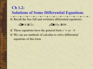
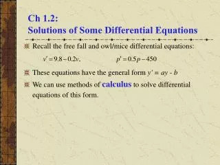
Ch 1.2: Solutions of Some Differential Equations. Recall the free fall and owl/mice differential equations: These equations have the general form y ' = ay - b We can use methods of calculus to solve differential equations of this form. Example 1: Mice and Owls (1 of 3).

E N D
Ch 1.2: Solutions of Some Differential Equations • Recall the free fall and owl/mice differential equations: • These equations have the general form y' = ay - b • We can use methods of calculus to solve differential equations of this form.
Example 1: Mice and Owls (1 of 3) • To solve the differential equation we use methods of calculus, as follows (note what happens when p = 900). • Thus the solution is where k is a constant.
Example 1: Integral Curves (2 of 3) • Thus we have infinitely many solutions to our equation, since k is an arbitrary constant. • Graphs of solutions (integral curves) for several values of k, and direction field for differential equation, are given below. • Choosing k = 0, we obtain the equilibrium solution, while for k 0, the solutions diverge from equilibrium solution.
Example 1: Initial Conditions (3 of 3) • A differential equation often has infinitely many solutions. If a point on the solution curve is known, such as an initial condition, then this determines a unique solution. • In the mice/owl differential equation, suppose we know that the mice population starts out at 850. Then p(0) = 850, and
Solution to General Equation • To solve the general equation (a ≠0) we use methods of calculus, as follows (y ≠b/a). • Thus the general solution is where k is a constant (k = 0 -> equilibrium solution). • Special case a = 0: the general solution is y = -bt + c
Initial Value Problem • Next, we solve the initial value problem (a ≠0) • From previous slide, the solution to differential equation is • Using the initial condition to solve for k, we obtain and hence the solution to the initial value problem is
Equilibrium Solution • Recall: To find equilibrium solution, set y' = 0 & solve for y: • From previous slide, our solution to initial value problem is: • Note the following solution behavior: • If y0 = b/a, then y is constant, with y(t) = b/a • If y0 > b/a and a > 0, then y increases exponentially without bound • If y0 > b/a and a < 0, then y decays exponentially to b/a • If y0 < b/a and a > 0, then y decreases exponentially without bound • If y0 < b/a and a < 0, then y increases asymptotically to b/a