Module 2.7 Estimation of uncertainties
680 likes | 869 Vues
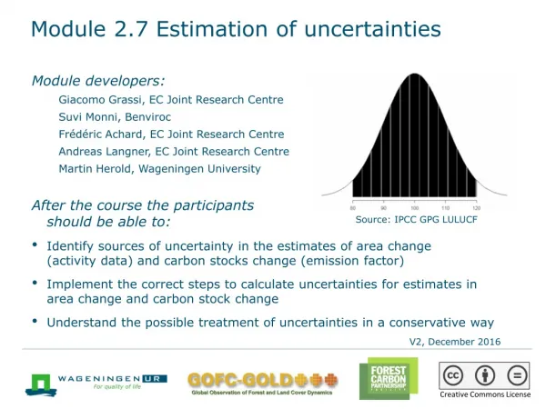
Module 2.7 Estimation of uncertainties. Module developers: Giacomo Grassi, EC Joint Research Centre Suvi Monni, Benviroc Frédéric Achard, EC Joint Research Centre Andreas Langner, EC Joint Research Centre Martin Herold, Wageningen University

Module 2.7 Estimation of uncertainties
E N D
Presentation Transcript
Module 2.7 Estimation of uncertainties Module developers: Giacomo Grassi, EC Joint Research Centre Suvi Monni, Benviroc Frédéric Achard, EC Joint Research Centre Andreas Langner, EC Joint Research Centre Martin Herold, Wageningen University After the course the participants should be able to: Identify sources of uncertainty in the estimates of area change (activity data) and carbon stocks change (emission factor) Implement the correct steps to calculate uncertainties for estimates in area change and carbon stock change Understand the possible treatment of uncertainties in a conservative way Source: IPCC GPG LULUCF V2, December 2016 Creative Commons License
Background material • GOFC-GOLD. 2014. Sourcebook. Section 2.7. • IPCC. 2003. Good Practice Guidance for Land Use, Land-Use Change, and Forestry. Ch. 5.2, “Identifying and Quantifying Uncertainties.” • IPCC. 2006. 2006 IPCC Guidelines for National Greenhouse Gas Inventories, vol. 1, ch. 3, “Uncertainties.” • GFOI. 2014. Integrating Remote-sensing and Ground-based Observations for Estimation of Emissions and Removals of Greenhouse Gases in Forests: Methods and Guidance from the Global Forest Observation Initiative (MGD). Sections 3.7 and 4.
Outline of lecture • Importance of identifying uncertainties • General concepts • Uncertainties in area-change estimates • Uncertainties in carbon stocks change estimates • Combination of uncertainties
Outline of lecture • Importance of identifying uncertainties • General concepts • Uncertainties in area-change estimates • Uncertainties in carbon stocks change estimates • Combination of uncertainties
Uncertainty in IPCC and UNFCCC context • Uncertainty is the lack of knowledge of the true value of a parameter (e.g., area and carbon stock estimates in REDD+ context) • Assessing uncertainty is fundamental in the IPCC and UNFCCC contexts: the IPCC defines greenhouse gas (GHG) inventories consistent with “good practice” as those which “contain neither over- nor underestimates so far as can be judged, and in which uncertainties are reduced as far as practicable.”
Importance of identifying uncertainties • A correct identification and quantification of the various sources of uncertainty helps to assess the robustness of any GHG inventory (including REDD+ estimates) and prioritize efforts for their further development. • In the accounting context, information on uncertainty can also be used to develop conservative REDD+ estimates, to ensure that reductions in emissions or increases in removals are not overestimated.
Aim of this module: Uncertainty estimation • Building on the IPCC (2003) guidance, this module aims to provide some basic elements for the identification, quantification, and combination of uncertainties for the estimates of: - Area and area changes (the activity data, AD) - Carbon stocks and carbon stock changes (the emission factors, EF)
Outline of lecture • Importance of identifying uncertainties • General concepts • Uncertainties in area-change estimates • Uncertainties in carbon stocks change estimates • Combination of uncertainties
Systematic errors and random errors (1/2) • Uncertainty consists of two components: • Bias or systematic error (lack of accuracy) occurs, e.g., due to flaws in the measurements or sampling methods or due to use of an EF that is not suitable • Random error (lack of precision) is a random variation above or below a mean value. It cannot be fully avoided but can be reduced by, for example, increasing the sample size. Accuracy: agreement between estimates and exact or true values Precision: agreement among repeated measurements or estimates (A) Accurate but not precise (B) Precise but not accurate (C) Accurate and precise
Systematic errors and random errors (2/2) • Systematic errors are to be avoided where possible , or quantified ex-post and removed. • Uncertainties that stem from random errors tend to cancel out each other at higher levels of aggregation. For example, estimates at national levels (e.g., total biomass, total forest area) usually* have a lower impact from random errors than estimates at regional levels. *Assuming that larger areashave greater sample sizes which, in turn, lead to greater precision and less uncertainty. However, for a smaller area and a larger area with the same sample size, the smaller area would probably have greater precision and less uncertainty, because the smaller area is likely more homogeneous. Thus sample size, and not the size of the area, is important.
95% Confidence interval • Uncertainty is usually expressed by a 95% confidence interval: • 95% of confidence intervals constructed using samples obtained with the same sampling design will include the true value. • If the area of forest land converted to cropland (mean value) is 100 ha, with a 95% confidence interval ranging from 80 to 120 ha, the uncertainty in the area estimate is ±20%. • The 2.5th percentile is 80 and the 97.5th percentile is 120. 120 100 110 80 90 Source: IPCC GPGLULUCF
Correlation • Correlation means dependency between parameters: • The “Pearson correlation coefficient” assumes values between [-1, +1] • Correlation coefficient of +1 means a perfect positive correlation • If the variables are independent of each other, the correlation coefficient is 0
Trend uncertainty • The trenddescribes the change of emissions or removals between two points in time. • Trend uncertainty describes the uncertainty in the change of emissions or removals. Trend uncertainty is sensitive to the correlation between parameter estimates used to estimate emissions or removals for two points in time. • Trend uncertainty is expressed as percentage points. For example, if the trend is +5% and the 95% confidence interval of the trend is +3 to +7%, we can say that trend uncertainty is ±2% points.
Outline of lecture • Importance of identifying uncertainties • General concepts • Uncertainties in area-change estimates • Uncertainties in carbon stocks change estimates • Combination of uncertainties
Uncertainties in area changes • In REDD+ context, an estimate of area and/or area change typically results from analysis of a remote-sensing-based map. • Such maps are subject to classification errors that induce bias into estimations. • A suitable approach is to assess the accuracy of the map and use the results of the accuracy assessment to adjust the area estimates. • Most image classification methods have parameters that can be tuned to reduce uncertainties. A good tuning reduces bias, but has a certain degree of subjectivity.
Accuracy assessment of land cover and changes (1/4) Use of accuracy assessment results for area estimation • The aim of the accuracy assessment is to characterize the frequency of errors (omission and commission) for each land cover class. • Differences in these two errors may be used to adjust area estimates and also to estimate the uncertainties (confidence intervals) for the areas for each class. • Adjusting area estimates on the basis of a rigorous accuracy assessment represents an improvement over simply reporting the areas of map classes.
Accuracy assessment of land cover and changes (2/4) • For land-cover maps the accuracy of remote sensing data (single-date) may be assessed with widely accepted methods. • These methods involve assessing the accuracy of a map using independent reference data (of greater quality than the map) to obtain—by land-cover class or by region—the overall accuracy, and: • Errors of omission (excluding an area from a category to which it does truly belongs, i.e., area underestimation) • Errors of commission (including an area in a category to which it does not truly belong, i.e., area overestimation)
Accuracy assessment of land cover and changes (3/4) • Example of accuracy measures for the forest class: • Error of commission: (13+45)/293 = 19.80% • Error of omission: (25+3)/263 = 10.65% • User’s accuracy: 235/293 = 80.20% • Producer’s accuracy: 235/263 = 89.35 • Overall accuracy = (235+187+215+92+75)/986 = 81.54%
Accuracy assessment of land cover and changes (4/4) For land-cover changes, additional considerations apply: • It is usually more difficult to obtain suitable, multitemporal reference data of greater quality to use as the basis of the accuracy assessment, particularly for historical time frames. • Since the changed classes are often small proportions of landscapes, it is easier to assess errors of commission (by examining small areas identified as changed) than errors of omission (by examining large area identified as unchanged). • Other errors such as geo-location of multitemporal datasets and inconsistencies in processing/analysis and in cartographic/ thematic standards are exaggerated and more frequent in change assessments.
Sources of uncertainty Different components of the monitoring system affect the quality of the estimates, including: • Quality and suitability of satellite data (i.e., in terms of spatial, spectral, and temporal resolution) • Radiometric / geometric preprocessing (correct geolocation) • Cartographic standards (i.e., land category definitions and MMU) • Interpretation procedure (algorithm or visual interpretation) • Postprocessing of the map products (i.e., dealing with no data, conversions, integration with different data formats) • Availability of reference data (e.g., ground truth data) for evaluation and calibration of the system
Addressing sources of uncertainty Many of these sources of uncertainty can be addressed using widely accepted data and approaches: • Suitable of satellite data: Landsat-type data, for example, have been proven useful for national-scale land cover changes for MMU of 1 ha • Data quality: suitable preprocessing for most regions provided by some data providers (i.e., global Landsat Geocover) • Consistent and transparent mapping: same cartographic and thematic standards and accepted interpretation methods should be applied transparently using expert interpreters The accuracy assessment should provide measures of thematic accuracy and confidence intervals for estimates of activity data
Errors in area-change estimates: Example Why errors in area-change estimates are more frequent than errors in area estimates Map at time 1 Map at time 2 Overlap (change) Omission error (forest reported as nonforest)Commission error (nonforest reported as forest)False afforestation False deforestation
Constructing area-change maps Two general approaches for constructing area-change maps: • Direct classification entails construction of the map directly from a set of change training data and two or more sets of remotely sensed data. If it is possible, this is often preferred, also because it has only a single set of errors • Postclassificationentails construction of the map by comparing two separate land-cover maps, each constructed using single sets of land-cover training data and remotely sensed data. Often it is the only possible alternative because of the inability to observe the same locations on multiple occasions as is required to obtain change training data, insufficient numbers of change training observations, or a requirement to use an historical baseline map.
Reference data and training data • Reference datashould be distinguished from the training data. • If estimates of accuracy, land cover, or change are to be representative of entire areas of interest, the reference data must be acquired using a probability sampling design. • The nature of the reference data depends on the method used to construct the map: • For maps constructed using direct classification, the reference data must consist of observations of change based on two dates for the same sample locations. • For maps constructed using postclassification, reference data may consist of either the same reference data as for maps constructed using direct classification or for two dates, each at different locations.
Elements for a robust accuracy assessment For robust accuracy assessment of land cover or land-cover change maps and estimates, statistically rigorous validations include three components: • Sampling design • Response design • Analysis design
Sampling design • Protocol for selecting the locations at which the reference data are obtained: It includes specification of the sample size, sample locations, and the reference assessment units (i.e., pixels or image blocks). • Stratified sampling should be used for rare classes (e.g., change categories). • Systematic sampling with a random starting point is generally more efficient than simple random sampling and is also more traceable.
Response design • Protocols used to determine the reference or ground condition classes and the definition of agreement for comparing the map classes to the reference classes. • Reference information should come from data of greater quality than the map labels; ground observations are generally considered the standard, although finer resolution remotely sensed data are also used. • Consistency and compatibility in thematic definitions and interpretation are required to compare reference and map data.
Analysis design • It includes estimators (statistical formulas) and analysis procedures for accuracy estimation and reporting.The estimators must be consistent with the sampling design. • Comparisons of map and reference data produce a suite of statistical estimates including error matrices, class-specific accuracies (of commission and omission error), area and area-change estimates, and associated variances and confidence intervals.
Considerations for implementation and reporting • The techniques described rely on probability sampling designs and the availability of suitable reference data. Such approach may not be achievable, in particular for historical land changes. • In the early stages of developing a national monitoring system, the verification efforts should help to build confidence. Greater experience (i.e., improving knowledge of source and magnitude of potential errors) will help reducing the uncertainties. • If no accuracy assessment is possible, it is recommended to perform, as a minimum, a consistency assessment (i.e., reinterpretation of small samples in an independent manner) which may provide information of the quality of the estimates.
Building confidence in estimates Information obtained without a proper probability sample design can still be useful to build confidence in the estimates, e.g.: • Spatially-distributed confidence values provided by the interpretation • Systematic qualitative examinations of the map and comparisons (qualitative / quantitative) with other maps • Review by local and regional experts • Comparisons with non-spatial and statistical data Any uncertainty bound should be treated conservatively to avoid producing a benefit for the country (overestimation of removals or of emissions reductions)
Outline of lecture • Importance of identifying uncertainties • General concepts • Uncertainties in area-change estimates • Uncertainties in carbon stocks change estimates • Combination of uncertainties
Uncertainties in carbon stock changes • Assessing uncertainties of the estimates of C stocks and C stocks changes is usually more challenging (and often subjective) than estimating uncertainties of the area and area changes • According to the literature, the overall uncertainty for C stocks estimates is usually larger than the uncertainty for area estimates. However, when looking at changes (i.e. trends) in C stocks and areas, the picture may change, depending on possible correlation of errors (see later)
Random errors and systematic errors • Uncertainty of carbon stocks can be caused by both random errorsand systematic errors, butsometimes it may be difficult to distinguish between the two. Representa-tiveness Random errors (affecting precision) Systematic errors (affecting accuracy) Conversion of tree measurement to biomass (allometric equations or BEFs) completeness sampling errors (plot size/number) Instrument imprecision/bias
Uncertainties due to random errors • Instrumental imprecision (noise, wrong handling, etc.) • Sampling errors (i.e., plot size and number), common with high natural variation of biomass in tropical forests Biomass depends on temperature, precipitation, forest type and species, stratification, spatial scale, natural and human disturbances, soil type, and soil nutrients.
Conversion of tree measurement to biomass • Allometric model or biomass expansion factors (BEFs): • Selection of best-fitting allometric model for respective forest type ≈ 20% error of tree AGB estimate • Overall: • Uncertainties on plot level (at 95% CI*): 5% to 30% • Average range of AGB of IPCC: -60% to +70% *CI = confidence interval.
Dealing with uncertainties due to random errors • If feasible: increase sample size (maybe problematic) • High tree biodiversity regional/pan-tropical allometric models are better than site-specific models (error ±5%)Dry forest stands: - AGB = exp(-2.187 + 0.916 x ln(pD2H)) ≡ 0.112 x (pD2H)0.916- AGB = p x exp(-0.667 + 1.784ln(D) + 0.207(ln(D))2– 0.0281(ln(D))3)Moist forest stands:- AGB = exp(-2.977 + ln(pD2H)) ≡ 0.0509 x pD2H- AGB = p x exp(-1.499 + 2.148ln(D) + 0.207(ln(D))2– 0.0281(ln(D))3) Equations from Chave et al., 2005 Having H (height), estimates are more accurate
Further regional/pan-tropical allometric models • (error ±5%)Moist mangrove forest stands: - AGB = exp(-2.977 + ln(pD2H)) ≡ 0.0509 x pD2H- AGB = p x exp(-1.349 + 1.980ln(D) + 0.207(ln(D))2– 0.0281(ln(D))3)Wetforest stands:- AGB = exp(-2.557 + 0.940 x ln(pD2H)) ≡ 0.0776 x (pD2H)0.940- AGB = p x exp(-1.239 + 1.980ln(D) + 0.207(ln(D))2– 0.0281(ln(D))3) AGB = aboveground biomass in kg; D = diameter in cm; p = oven-dry wood over green volume in g/cm^-3; H = height of tree in m; ≡ = mathematical identity
Uncertainties due to systematic errors • Completeness of carbon pools: aboveground biomass, belowground biomass, soil organic carbon, deadwood, litter: • Literature suggests that for deforestation, ≈15% of emissions may come from dead organic and ≈ 25-30% may come from soils (more if organic soils) • However, these pools are often not included when calculating emission factors, due to lack of data
Dealing with uncertainties due to carbon pool completeness • All “significant” pools and activities should be included: • First, “Key categories” (KC) (i.e., categories/ activities contributing substantially to the national GHG inventory) should be identified following IPCC guidance (IPCC, 2006, V4, Ch1.1.3) • Within a KC, a pool is “significant” if it accounts for >25-30% of emissions from the category • Pools may be omitted under principle of conservativeness • Furthermore, emissions/removals from KC and significant pools should be estimated with Tier 2 or 3 methods,* which are assumed less uncertain than tier 1 *National circumstances (e.g., documented lack of resources) may justify use of Tier 1 for KC
Representativeness of the sampling plots • High variation of biomass content within tropical forests a nonrepresentative sample may introduce a significant bias
Dealing with uncertainties due to representativeness • Sound statistical sampling necessary in “hotspots” • Distribution of samples across major soil/topographic gradients of landscape, e.g., 20 plots (each 0.25ha) or one sample of 5ha may allow landscape-scale AGB estimation with ±10% (95% CI) • If geographic position known, global biomass maps (1km Saatchi / 500m Baccini) can be used for estimating AGB • If geographic position unknown, global biomass maps can be used to derive improved Tier 1 data values
Error propagation of AGB estimation (Chave et al. 2004) For Central Panama: (gravity)
Examples of uncertainties of recent AGB global maps (1/3) Saatchi map at 95% CI: • Overall AGB uncertainty at pixel-level (averaged)±30% (±6% to ±53%) • Regional uncertainties:America ±27%; Africa ±32%Asia ±33% • Total C stock uncertaintyat pixel-level (averaged)±38%; ±5% (10,000ha); ±1% (>1,000,000ha)
Examples of uncertainties of recent AGB global maps (2/3) Baccini map at 95% CI: • Regional uncertaintiesfor carbon stocks:America ±7.1%; Africa ±13.2%Asia ±6.5%
Examples of uncertainties of recent AGB global maps (3/3) Difference between Baccini and Saatchi maps: • Recent analysis shows locallysignificant differences, but atregion-scale level results are comparable
Outline of lecture • Importance of identifying uncertainties • General concepts • Uncertainties in area-change estimates • Uncertainties in carbon stocks change estimates • Combination of uncertainties
Combination of uncertainties • The uncertainties in individual parameters can be combined using either: • Error propagation (IPCC Tier 1), which is easy to implement using a spreadsheet tool; certain conditions have to be fulfilled so that it can be used. • Monte Carlo simulation (IPCC Tier 2), based on modelling and requiring more resources to be implemented; it can be applied to any data or model.
Tier 1 level assessment (1/3) Tier 1 should preferably be used only when: • Estimation of emissions and removals is based on addition, subtraction, and multiplication • There are no correlations across categories (or categories are aggregated in a way that correlations are unimportant • Relative ranges of uncertainty in the emission factors and area estimates are the same in years 1 and 2 • No parameter has an uncertainty > than about ±60% • Uncertainties are symmetric and follow normal distribution Even in the case that not all of the conditions are fulfilled, the Tier 1 method can be used to obtain approximate results If asymmetric distributions take higher absolute value
Tier 1 level assessment (2/3) • Equation for multiplication: • Equation foraddition and substraction:
Tier 1 level assessment (3/3) Examples of combination of uncertainties with Tier 1 Multiplication Addition