KDD Overview
KDD Overview. Xintao Wu. What is data mining?. Data mining is extraction of useful patterns from data sources, e.g., databases, texts, web, images, etc. Patterns must be: valid, novel, potentially useful, understandable. Classic data mining tasks. Classification:


KDD Overview
E N D
Presentation Transcript
KDD Overview Xintao Wu
What is data mining? • Data mining is • extraction of useful patterns from data sources, e.g., databases, texts, web, images, etc. • Patterns must be: • valid, novel, potentially useful, understandable
Classic data mining tasks • Classification: mining patterns that can classify future (new) data into known classes. • Association rule mining mining any rule of the form X Y, where X and Y are sets of data items. • Clustering identifying a set of similarity groups in the data
Classic data mining tasks (contd) • Sequential pattern mining: A sequential rule: A B, says that event A will be immediately followed by event B with a certain confidence • Deviation detection: discovering the most significant changes in data • Data visualization CS583, Bing Liu, UIC
Why is data mining important? • Huge amount of data • How to make best use of data? • Knowledge discovered from data can be used for competitive advantage. • Many interesting things that one wants to find cannot be found using database queries, e.g., “find people likely to buy my products”
Related fields • Data mining is an multi-disciplinary field: Machine learning Statistics Databases Information retrieval Visualization Natural language processing etc.
Association Rule: Basic Concepts • Given: (1) database of transactions, (2) each transaction is a list of items (purchased by a customer in a visit) • Find: all rules that correlate the presence of one set of items with that of another set of items • E.g., 98% of people who purchase tires and auto accessories also get automotive services done
Rule Measures: Support and Confidence Customer buys both Customer buys diaper • Find all the rules X Y with minimum confidence and support • support, s, probability that a transaction contains {X Y } • confidence, c,conditional probability that a transaction having X also contains Y Customer buys beer Let minimum support 50%, and minimum confidence 50%, we have • A C (50%, 66.6%) • C A (50%, 100%)
Applications • Market basket analysis: tell me how I can improve my sales by attaching promotions to “best seller” itemsets. • Marketing: “people who bought this book also bought…” • Fraud detection: a claim for immunizations always come with a claim for a doctor’s visit on the same day. • Shelf planning: given the “best sellers,” how do I organize my shelves?
Mining Frequent Itemsets: the Key Step • Find the frequent itemsets: the sets of items that have minimum support • A subset of a frequent itemset must also be a frequent itemset • i.e., if {AB} isa frequent itemset, both {A} and {B} should be a frequent itemset • Iteratively find frequent itemsets with cardinality from 1 to k (k-itemset) • Use the frequent itemsets to generate association rules.
The Apriori Algorithm • Join Step: Ckis generated by joining Lk-1with itself • Prune Step: Any (k-1)-itemset that is not frequent cannot be a subset of a frequent k-itemset • Pseudo-code: Ck: Candidate itemset of size k Lk : frequent itemset of size k L1 = {frequent items}; for(k = 1; Lk !=; k++) do begin Ck+1 = candidates generated from Lk; for each transaction t in database do increment the count of all candidates in Ck+1 that are contained in t Lk+1 = candidates in Ck+1 with min_support end returnkLk;
The Apriori Algorithm — Example Database D L1 C1 Scan D C2 C2 L2 Scan D L3 C3 Scan D
Example of Generating Candidates • L3={abc, abd, acd, ace, bcd} • Self-joining: L3*L3 • abcd from abc and abd • acde from acd and ace • Pruning: • acde is removed because ade is not in L3 • C4={abcd}
Criticism to Support and Confidence • Example 1: (Aggarwal & Yu, PODS98) • Among 5000 students • 3000 play basketball • 3750 eat cereal • 2000 both play basket ball and eat cereal • play basketball eat cereal [40%, 66.7%] is misleading because the overall percentage of students eating cereal is 75% which is higher than 66.7%. • play basketball not eat cereal [20%, 33.3%] is far more accurate, although with lower support and confidence
Criticism to Support and Confidence (Cont.) • We need a measure of dependent or correlated events • If Corr < 1 A is negatively correlated with B (discourages B) • If Corr > 1 A and B are positively correlated • P(AB)=P(A)P(B) if the itemsets are independent. (Corr = 1) • P(B|A)/P(B) is also called the lift of rule A => B (we want positive lift!)
Classification—A Two-Step Process • Model construction: describing a set of predetermined classes • Each tuple/sample is assumed to belong to a predefined class, as determined by the class label attribute • The set of tuples used for model construction: training set • The model is represented as classification rules, decision trees, or mathematical formulae • Model usage: for classifying future or unknown objects • Estimate accuracy of the model • The known label of test sample is compared with the classified result from the model • Accuracy rate is the percentage of test set samples that are correctly classified by the model • Test set is independent of training set, otherwise over-fitting will occur
Classification by Decision Tree Induction • Decision tree • A flow-chart-like tree structure • Internal node denotes a test on an attribute • Branch represents an outcome of the test • Leaf nodes represent class labels or class distribution • Decision tree generation consists of two phases • Tree construction • At start, all the training examples are at the root • Partition examples recursively based on selected attributes • Tree pruning • Identify and remove branches that reflect noise or outliers • Use of decision tree: Classifying an unknown sample • Test the attribute values of the sample against the decision tree
Some probability... • Entropy info(S) = - (freq(Ci,S)/|S|) log (freq(Ci,S)/|S|) S = cases freq(Ci,S) = # cases in S that belong to Ci Prob(“this case belongs to Ci”) = freq(Ci,S)/|S| • Gain Assume attribute A divide set T into Ti. i =1,…,m info(T_new) = |Ti|/S info(Ti) gain(A) = info (T) - info(T_new)
5/14 (-2/5 log(2/5)-3/5 log(3/5))+ 7/14(-4/7log(4/7)-3/7 log(3/7)) 4/14 (-4/4 log(4/4)) + +7/14(-5/7log(5/7)-2/7log(2/(7)) 5/14 (-3/5 log(3/5) - 2/5 log(2/5)) Example Info(T) (9 play, 5 don’t) info(T) = -9/14log(9/14)- 5/14log(5/14) = 0.94 (bits) Test: outlook infoOutlook = Test Windy infowindy= gainOutlook = 0.94-0.64= 0.3 = 0.278 gainWindy = 0.94-0.278= 0.662 = 0.64 (bits) Windy is a better test
Bayesian Classification: Why? • Probabilistic learning: Calculate explicit probabilities for hypothesis, among the most practical approaches to certain types of learning problems • Incremental: Each training example can incrementally increase/decrease the probability that a hypothesis is correct. Prior knowledge can be combined with observed data. • Probabilistic prediction: Predict multiple hypotheses, weighted by their probabilities • Standard: Even when Bayesian methods are computationally intractable, they can provide a standard of optimal decision making against which other methods can be measured
Bayesian Theorem • Given training data D, posteriori probability of a hypothesis h, P(h|D) follows the Bayes theorem • MAP (maximum posteriori) hypothesis • Practical difficulty: require initial knowledge of many probabilities, significant computational cost
Naïve Bayes Classifier (I) • A simplified assumption: attributes are conditionally independent: • Greatly reduces the computation cost, only count the class distribution.
Naive Bayesian Classifier (II) • Given a training set, we can compute the probabilities
(2/9x 3/9 x 3/9 x Example E ={outlook = sunny, temp = [64,70], humidity= [65,70], windy = y} = {E1,E2,E3,E4} Pr[“Play”/E] = (Pr[E1/Play] x Pr[E2/Play] x Pr[E3/Play] x Pr[E4/Play] x Pr[Play]) / Pr[E] = 4/9x 9/14)/Pr[E] = 0.007/Pr[E] Pr[“Don’t”/E] = (3/5 x 2/5 x 1/5 x 3/5 x 5/14)/Pr[E] = 0.010/Pr[E] With E: Pr[“Play”/E] = 41 %, Pr[“Don’t”/E] = 59 %
Bayesian Belief Networks (I) Family History Smoker (FH, S) (FH, ~S) (~FH, S) (~FH, ~S) LC 0.7 0.8 0.5 0.1 LungCancer Emphysema ~LC 0.3 0.2 0.5 0.9 The conditional probability table for the variable LungCancer PositiveXRay Dyspnea Bayesian Belief Networks
What is Cluster Analysis? • Cluster: a collection of data objects • Similar to one another within the same cluster • Dissimilar to the objects in other clusters • Cluster analysis • Grouping a set of data objects into clusters • Clustering is unsupervised classification: no predefined classes • Typical applications • As a stand-alone tool to get insight into data distribution • As a preprocessing step for other algorithms
Requirements of Clustering in Data Mining • Scalability • Ability to deal with different types of attributes • Discovery of clusters with arbitrary shape • Minimal requirements for domain knowledge to determine input parameters • Able to deal with noise and outliers • Insensitive to order of input records • High dimensionality • Incorporation of user-specified constraints • Interpretability and usability
Major Clustering Approaches • Partitioning algorithms: Construct various partitions and then evaluate them by some criterion • Hierarchy algorithms: Create a hierarchical decomposition of the set of data (or objects) using some criterion • Density-based: based on connectivity and density functions • Grid-based: based on a multiple-level granularity structure • Model-based: A model is hypothesized for each of the clusters and the idea is to find the best fit of that model to each other
Partitioning Algorithms: Basic Concept • Partitioning method: Construct a partition of a database D of n objects into a set of k clusters • Given a k, find a partition of k clusters that optimizes the chosen partitioning criterion • Global optimal: exhaustively enumerate all partitions • Heuristic methods: k-means and k-medoids algorithms • k-means (MacQueen’67): Each cluster is represented by the center of the cluster • k-medoids or PAM (Partition around medoids) (Kaufman & Rousseeuw’87): Each cluster is represented by one of the objects in the cluster
The K-Means Clustering Method • Given k, the k-means algorithm is implemented in 4 steps: • Partition objects into k nonempty subsets • Compute seed points as the centroids of the clusters of the current partition. The centroid is the center (mean point) of the cluster. • Assign each object to the cluster with the nearest seed point. • Go back to Step 2, stop when no more new assignment.
The K-Means Clustering Method • Example
Comments on the K-Means Method • Strength • Relatively efficient: O(tkn), where n is # objects, k is # clusters, and t is # iterations. Normally, k, t << n. • Often terminates at a local optimum. The global optimum may be found using techniques such as: deterministic annealing and genetic algorithms • Weakness • Applicable only when mean is defined, then what about categorical data? • Need to specify k, the number of clusters, in advance • Unable to handle noisy data and outliers • Not suitable to discover clusters with non-convex shapes
Step 0 Step 1 Step 2 Step 3 Step 4 agglomerative (AGNES) a a b b a b c d e c c d e d d e e divisive (DIANA) Step 3 Step 2 Step 1 Step 0 Step 4 Hierarchical Clustering • Use distance matrix as clustering criteria. This method does not require the number of clusters k as an input, but needs a termination condition
More on Hierarchical Clustering Methods • Major weakness of agglomerative clustering methods • do not scale well: time complexity of at least O(n2), where n is the number of total objects • can never undo what was done previously • Integration of hierarchical with distance-based clustering • BIRCH (1996): uses CF-tree and incrementally adjusts the quality of sub-clusters • CURE (1998): selects well-scattered points from the cluster and then shrinks them towards the center of the cluster by a specified fraction • CHAMELEON (1999): hierarchical clustering using dynamic modeling
Density-Based Clustering Methods • Clustering based on density (local cluster criterion), such as density-connected points • Major features: • Discover clusters of arbitrary shape • Handle noise • One scan • Need density parameters as termination condition • Several interesting studies: • DBSCAN: Ester, et al. (KDD’96) • OPTICS: Ankerst, et al (SIGMOD’99). • DENCLUE: Hinneburg & D. Keim (KDD’98) • CLIQUE: Agrawal, et al. (SIGMOD’98)
Grid-Based Clustering Method • Using multi-resolution grid data structure • Several methods • STING(a STatistical INformation Grid approach) by Wang, Yang and Muntz (1997) • WaveCluster by Sheikholeslami, Chatterjee, and Zhang (VLDB’98) • CLIQUE: Agrawal, et al. (SIGMOD’98) • Self-Similar Clustering Barbará & Chen (2000)
Model-Based Clustering Methods • Attempt to optimize the fit between the data and some mathematical model • Statistical and AI approach • Conceptual clustering • A form of clustering in machine learning • Produces a classification scheme for a set of unlabeled objects • Finds characteristic description for each concept (class) • COBWEB (Fisher’87) • A popular a simple method of incremental conceptual learning • Creates a hierarchical clustering in the form of a classification tree • Each node refers to a concept and contains a probabilistic description of that concept
COBWEB Clustering Method A classification tree
Summary • Association rule and frequent set mining • Classification: decision tree, bayesian network, SVM, etc. • Clustering algorithms can be categorized into partitioning methods, hierarchical methods, density-based methods, grid-based methods, and model-based methods • Other data mining tasks