Download
1 / 29
340 likes | 764 Vues
Discrete Differential-Geometry Operators for Triangulated 2-Manifolds. Mark Meyer, Mathieu Desbrun, Peter Schroder, and Alan H. Barr Presented by Shadi Ashnai. Overview. Motivation Definitions Derive differential geometry operators Accuracy analysis Generalization. Applications.

E N D
Discrete Differential-Geometry Operators for Triangulated 2-Manifolds Mark Meyer, Mathieu Desbrun, Peter Schroder, and Alan H. Barr Presented by Shadi Ashnai
Overview • Motivation • Definitions • Derive differential geometry operators • Accuracy analysis • Generalization
Applications • Mesh quality • Mesh simplification • Mesh modeling • Denoising (a) mean curvature plot (b) principal directions (c-d) feature preserving denoising
Previous Works • n(p) = weighted average of the adjacent face normals • Some introduced weights are: • Incident adjacent angles: independent of the shape and length of the adjacent faces [Thurmer and Wuthrich 98] • Computed by assuming that surface can locally be approximated by a sphere [Max 99] • [Taubin 95] introduced a complete derivation of surface properties approximating curvature tensors for polyhedral surface • [Hamann 93] simple way to determine principal curvature and direction using least-squared paraboloid fitting • No easy way to selecting an appropriate tangent plane
Definitions • n : Normal vector • N() : normal curvature for unit direction • 1 , 2 : principal curvatures • e1 , e2 : principal directions • H : mean curvature • G: gaussian curvature
Definitions (cntd.) • H (mean curvature): • Mean curvature normal (Laplace-Beltrami) operator: • G (gaussian curvature):
Discrete Geometry Attributes • Mesh as linear approximation of an artibrary surface • Define geometric quantities: • as spatial averages around each vertex • Converge to the pointwise definitions knowing that: • The mesh is a good approximation of the initial surface • The averages are made consistently • The triangle mesh is non-degenerate • etc. • Example (Gaussian curvature):
Local Regions • Select a linear finite element on each triangle • Circumcenter - AVoronoi • Barycenter - ABarycenter • Generally we do the calculation with AM
Discrete Mean Curvature • We compute “mean curvature normal”, know as Laplace-Beltrami operator. • Once we compute this operator: • H is half the magnitude of K • n is the normalized K
Integral of “Mean Curvature Normal” • Using conromal space parameters u,v • Using Gauss’s theorm:
Minimizing Error Bounds • Compare local spatial average with actual value: • Minimizing E: • Use voronoi region that minimizes ||x-xi|| (by definition) • Sample with respect to curvature such that Ci’s vary slowly from patch to patch (assume)
Voronoi Region Area • For non-obtuse triangle: • In presence of obtuse angles: • Use mixed regions
Mean curvature normal • H: half the magnitude of Κ(xi) • n: • normalized Κ(xi), if H<>0 • Average of the 1-ring face normals, if H=0
Integral of the Gaussian curvature • Gauss-Bonnet theorm: • Discrete model: • For voronoi region:
Gaussian curvature • We can use mixed regions the same as used for H and the region still satisfies the Gauss-Bonnet theorm
Discrete Principal Curvatures G=12 H=(1+2)/2
An estimate of the normal curvature in direction xixj Principal Directions • Mean curvature as a quadrature of normal curvature samples:
Principal Directions • Mean curvature interpretation: • Use normal curvature samples to fully determine curvature tensor • Principal directions are eigenvectors of the curvature tensor
Least square fitting • Symmetric curvature tensor • For finding curvature in direction xixj: • Least square approximation:
Geometric Quality of Meshes (a) Loop surface from an 8-neighbor ring (b) Horse mesh (c-d) noisy scanned and smoothed head
Denoising (a) 3% noise added along the normal (b) Isotropic smoothing (c) Anisotropic smoothing
Generalization • 2D-manifolds in nD • Mean curvature normal: • generalize area and cot expressions for nD • Gaussian curvature operator: • still holds (independent of embedding) • 3D-manifolds in nD • Compute gradient of the 1-ring volume for Beltrami operator
Denoising of Arbitrary Fields (a) Original noisy vector field (b) Smoothed using Beltrami flow (c) Smoothed using anisotropic weighted flow