Permutation Procedures, Bootstrap Methods and the Jackknife
Permutation Procedures, Bootstrap Methods and the Jackknife. Bob Livezey Climate Services Division/OCWWS/NWS AMS Short Course on Significance Testing, Model Evaluation and Alternatives Seattle, January 11, 2004. Outline. Introduction Problems addressed What is being done, why, and how


Permutation Procedures, Bootstrap Methods and the Jackknife
E N D
Presentation Transcript
Permutation Procedures, Bootstrap Methods and the Jackknife Bob Livezey Climate Services Division/OCWWS/NWS AMS Short Course on Significance Testing, Model Evaluation and Alternatives Seattle, January 11, 2004
Outline • Introduction • Problems addressed • What is being done, why, and how • Resampling/rerandomization primer • Bootstrap/correlation example • Histograms, standard error, bias, confidence intervals • Significance test • Multivariate applications • Discussion examples • Livezey and Chen example • Serial correlation • Impact • Solutions • Summary
Introduction • Problems: A statistic has been estimated from a sample, we want to • know how confident we can be in the estimator and what its standard error and bias are, and • gauge the estimator against a null distribution we want to discount • What, why, and how. • Rather than using classical and/or analytical statistics we use brute force (Monte Carlo) computations to generate huge numbers of synthetic or fake samples. These samples form the basis for constructing sampling distributions of either the estimator itself or its null distribution to address respectively the two problems.
Introduction • What, why, and how. • It is not clear assumptions for usual approaches are satisfied. • Sample sizes are too small for satisfactory application of usual approaches. • It is not easy or possible to derive analytical descriptions of distributions for the estimator. • The inference problem is complicated.
Introduction • What, why, and how. • Resampling/rerandomization: Using the available sample to generate additional samples. • Statistical modeling: Fitting a model to the available sample and using the model to generate additional samples, another meaning for “Monte Carlo Method,” ex. is time series modeling.
Introduction • Take away knowledge: • Clear intuitive understanding of the basic problems, and whys and hows of computer intensive solutions to the problems. • Basic algorithms for permutation, bootstrap, and jackknife procedures and when to use. • The necessity to preserve spatial-temporal interdependence in applying methods. • Reference sources to build understanding and study more examples.
Comparison of Resampling Techniques • Most versatile. • Generally outperformed by others.
Resampling Examples • Mean DJF temperature in Eastern North Dakota for 10 moderate to strong El Nino years from a 60-year record. • Null hypothesis is that moderate to strong El Ninos do not impact DJF temperature in Eastern North Dakota. • Null distribution is for average of 10 DJFs chosen randomly.
Resampling Examples • Null distributions from permutation and bootstrap procedures: • Permutation: Shuffle the 60 years, relabel them, pull out the 10 relabeled El Nino years and average them (equivalent to random draw of 10 from 60 without replacement). Repeat huge (1000?) number of times. • Bootstrap: Shuffle a huge deck where the 60 years are replicated many, many times, take the first 60 and relabel (same as random draw of 10 from 60 with replacement). Repeat huge (1000?) number of times.
NULL RESAMPLING DISTRIBUTIONS (1000 samples) 10 Year Means of Eastern North Dakota DJF Temperature (1941-2000) Relative Frequency (%) 0.5º F Bins (Upper limits)
Resampling Examples • Distribution of 10 El Nino-year mean from bootstrap and jackknife procedures: • Bootstrap: Shuffle a huge deck where the 10 El Nino years are replicated many, many times and average the first 10 (equivalent to random draw of 10 from 10 with replacement). Repeat huge (1000?) number of times. • Jackknife: Delete one of 10 El Nino years from the sample and average the rest. Repeat for each of the 10 years. Produce 10 9-year means.
RESAMPLING DISTRIBUTIONS 10 Year Means of Eastern North Dakota DJF Temperature (1941-2000) Relative Frequency (%) 0.5º F Bins (Upper limits)
BOOTSTRAP DISTRIBUTIONS (1000 samples) 10 Year Means of Eastern North Dakota DJF Temperature (1941-2000) Relative Frequency (%) 0.5º F Bins (Upper limits)
Resampling Examples • Notes for permutation and bootstrap: • Random selection uses uniform distribution by assigning probability of 1/N (N is sample size) to each member of the sample being drawn from. • Number of replications depends on the distribution attribute and precision desired (ex. information about the tails).
Bootstrap Correlation Examples • Correlations between JFM temperature for CD93 (San Diego) and CD76 (Olympic Peninsula) and CD67 (Central Florida) are respectively 0.72 and -0.3. • Computed • 10,000-sample bootstrap histograms for both. Paired data were resampled with replacement. • 10,000-sample bootstrap null histogram for the corr(CD93,CD67). Each series separately resampled with replacement to form pairs.
BOOTSTRAP DISTRIBUTIONS (10000 Samples) Correlation (1950-1999) between JFM Temperatures at CD93 and CD67 Relative Frequency (%) Null Correlation (1950-1999) between JFM Temperatures at CD93 and CD67 .002 tail for corr -0.297 Correlation
Bootstrap Correlation Examples • Computed (continued) • For corr(CD93,CD76) • Standard error • Bias • 68% (plus/minus one in standard normal distribution) confidence intervals • Percentile method • Bias-corrected percentile method (see Efron and Gong)
BOOTSTRAP DISTRIBUTION (1000 SAMPLES) FOR CORRELATION (1950-1999)BETWEEN JFM TEMPERATURES AT CD93 and CD76 Correlation 0.717 Relative Frequency (%) Correlation
BOOTSTRAP DISTRIBUTION (10000 SAMPLES) FOR CORRELATION (1950-1999)BETWEEN JFM TEMPERATURES AT CD93 and CD76 Correlation 0.717 Bias 0.001 St. error 0.051 Conf. Limits: Percentile method Bias-corrected Relative Frequency (%) Correlation
Multivariate Applications • Sampling error for an estimator generally decreases as independent sample size increases. Ex. Florida January mean temperature. Start year Florida Jan Temperature (°F) Average
Multivariate Applications • Samples drawn from different locations and/or times may not be independent of each other, i.e. spatially and/or serial correlated. • Bootstrap and permutation resampling under the null hypothesis among such locations and/or times reduces or destroys this interdependence. • This leads to null distributions that are too narrow.
Multivariate Applications • Interdependencies must be preserved when resampling. • Ex. DJF skill score for CPC temperature forecasts at 100 locations over 10 winters. • Both forecasts and observations have considerable spatial correlation. • Incorrect strategy for null distribution is to form forecast/observation pairs by separately resampling with replacement 1000 pooled forecasts and 1000 pooled observations. • Correct strategy is to form pairs by separately resampling with replacement 10 pooled forecast maps and 10 pooled observation maps.
Multivariate Applications ● In climate studies a defining problem is the Livezey and Chen (1983) example; determine the statistical significance of correlation of the SOI time series to the full field of NH seasonal mean 700 mb heights. It will be used to illustrate: The effects of spatial correlation on the spread of a false signal distribution; Field significance.
Multivariate Applications Livezey and Chen (1983) estimated the probability that a map with a similar number of locally significant correlations could have been obtained by chance. They coined the term field significance for this probability.
Multivariate Applications Sampling distributions developed by repeatedly computing correlations with random series instead of SOI– statistic is count of passed significance tests; Distribution becomes narrower as the ratio of the domain size to signal scale increases (from C to A to B).
Serial Correlation • Zwiers (1990) example of impact. • Generated a multivariate statistic (dimension m, sample size 10) from a known null-distribution. Each m-variable is uncorrelated with the others but all have the same serial correlation. • Used a permutation procedure to develop the null distribution from the sample. • Tested the statistic against the constructed distribution at the 5% level. • Repeated the experiment many, many times. • Noted the percent of times the null hypothesis is rejected (should be near 5%).
Serial Correlation • Zwiers (1990) example continued. • Percent rejections • Serial correlation makes almost all of the tests worthless.
Serial Correlation • Remedies • Model the time series with an autoregressive model and use the model to generate samples. • Livezey and Chen could have done this with their SOI series. • Many meterological time series with the climatological seasonal cycle removed are well represented by a red noise (AR(1), damped persistence) model: • AR(1) model not appropriate for quasi-cyclical series, like MJO, QBO, etc. • See references in Livezey (1999) for more guidance.
Serial Correlation • Remedies continued • Use Moving-Blocks bootstrap • Idea is to preserve much of the serial correlation by resampling blocks of data of length L with replacement to build up the full series from N/L blocks. • There are N-L+1 blocks to choose from. • See Livezey (1999) for information (including references) for choosing L.
References • Basic sources • Diaconis, P., and B. Efron, 1983: Computer-intensive methods in statistics. Sci. Am.,248, 116-130. (Popular description.) • Efron, B., and G. Gong, 1983: A leisurely look at the bootstrap, the jackknife, and cross-validation. Am. Stat., 37, 36-48. (Basic strategies and algorithms.) • Efron, B., and R. Tibshirani, 1997: Improvements on cross-validation: the .632+ bootstrap method. J. Amer. Stat. Assoc., 92, 548-560. • Texts • Livezey, R. E., 1999: Chapter 9, Field intercomparison. Analysis of Climate Variability: Applications of Statistical Techniques, Second Updated and Extended Edition, Eds. H. von Storch and A. Navarra, Springer-Verlag, Berlin, 161-178. (Contains unlisted references.) • von Storch, H., and F. W. Zwiers, 1999: Statistical Analysis in Climate Research, Cambridge University Press, 484pp. • Wilks, D. S., 1995: Statistical Methods in the Atmospheric Sciences. Academic Press, 467pp.