Uncertainty Management In Rule Based Information Extraction Systems
220 likes | 395 Vues
Uncertainty Management In Rule Based Information Extraction Systems. Author Eirinaios Michelakis Rajasekar Krishnamurthy Peter J. Haas Shivkumar Vaithyanathan Presented By Anurag Kulkarni. Introduction. Rule based information extraction Need

Uncertainty Management In Rule Based Information Extraction Systems
E N D
Presentation Transcript
Uncertainty Management In Rule Based Information Extraction Systems Author Eirinaios Michelakis Rajasekar Krishnamurthy Peter J. Haas Shivkumar Vaithyanathan Presented By Anurag Kulkarni
Introduction • Rule based information extraction • Need • Uncertainty in extraction due to the varying precision associated with the rules used in a specific extraction task • Quantification of the Uncertainty for the extracted objects in Probabilistic databases(PDBs) • To improve recall of extraction tasks. • Types of Rule Based IE Systems • Trainable : rules are learned from data • Knowledge-engineered : rules are hand crafted by domain experts. User Defined Rules Unstructured Data (Any free Text) Structured Data (e.g. objects in the Database)
Keywords • Annotator : A coordinated set of rules written for a particular IE task • base annotators – operate only over raw text • derived annotators - operate over previously defined annotations • Annotations : Extracted objects • Rules • Consolidationrule (K): Special rule used to combine the outputs of the annotator rules. • Candidate-generation rules (R): each individual rule • Discard Rules: discard some candidates • Merge Rules: merge a set of candidates to produce a result annotation. • Confidence : probability of the associated annotation being correct • Span: An annotator identifies a set of structured objects in a body of text, producing a set of annotations. Annotation a = (s1, . . . , sn) is a tuple of spans. • Annotation: Person and PhoneNumber E.g. input text “. . . Greg Mann can be reached at 403-663-2817 . . .” s = “Greg Mann can be reached at 403-663-2817” s1 = ”Greg Mann” s2 = “403-663-2817”
Template For A Rule-based Annotator Algorithm 1: Template for a Rule-based Annotator
Need Of Probabilistic Framework • Simple associating an arbitrary confidence rating of, e.g., “high”, “medium”, or “low” with each annotation is insufficient. • Need of Confidence associated with Annotation • Use of confidence number • enable principled assessments of risk or quality in applications that use extracted data. • improve the quality of annotators themselves • associate a probability with each annotation to capture the annotator’s confidence that the annotation is correct. • Modified rule based tuple (R,K,L, C). where training data L = (LD,LL) LD set of training documents LL set of labels For example, a label might be represented as a tuple of the form (docID, s, Person), where s is the span corresponding to the Person annotation. C describes key statistical properties of the rules that comprise the annotator, • Modified Consolidate operator to include rule history • Modified procedure to include statistical model M
Problem Statement • q(r) = P(A(s) = 1 | R(s) = r,K(s) = 1) • q(r) as the confidence associated with the annotation • R(s) =R1(s),R2(s), . . . ,Rk(s) , Ri(s) = 1 if and only if rule Ri holds for span s or at least one sub-span of s • A(s) = 1 if and only if spans corresponds to a true annotation • H the set of possible rule histories, H = { 0, 1 }k and r ∈ H using Bayes’ rule p1(r) = P(R(s) = r | A(s) = 1,K(s) = 1) and p0(r) = P(R(s) = r | A(s) = 0,K(s) = 1) setting π = P(A(s) = 1 | K(s) = 1). Then again applying bayes rule yields q(r) = πp1 (r) /(πp1(r) + (1 − π)p0(r)) • Here we have converted the problem of estimating a collection of posterior • probabilities to the problem of estimating the distributions p0 and p1, Unfortunately, whereas this method typically works well for estimating π, the estimates for p0 and p1 can be quite poor. The problem is data sparsity because there are 2k different possible r values and only a limited supply of labeled training data.
Derivation Of Parametric Model • select a set C of important constraints that are satisfied by p1, and then to approximate p1 by the “simplest” distribution that obeys the constraints in C. • Following standard practice, we formalize the notion of “simplest distribution” as the distribution p satisfying the given constraints that has the maximum entropy value H(p), • where • Denoting by P the set of all probability distributions over H, we approximate p1 by the solution p to the maximization problem. maximize H(p) such that fc is the indicator function of that subset, so that fc(r) = 1 ac = computed directly from the training data L as Nc/N1. N1 is the number of spans s such that A(s) = 1 and K(s) = 1, and Nc is the number of these spans such that fc (R(s))= 1
Derivation Of Parametric Model cont. • Reformulate our maximum-entropy problem as a more convenient maximum-likelihood (ML) problem. • θ = { θc : c ∈ C } is the set of Lagrange multipliers for the original problem. To solve the inner maximization problem, take the partial derivative with respect to p(r) and set this derivative equal to 0, to obtain • where Z(θ) is normalizing constant that ensures Substituting value of p(r) in above equation • But assuming ac is estimated from the training data
Derivation Of Parametric Model cont. • Multiply the objective function by the constant N1, and change the order of summation to find that solving the dual problem is equivalent to solving the optimization problem • The triples {A(s),K(s),R(s): s ∈ S } are mutually independent for any set S of distinct spans, and denote by S1 the set of spans such that A(s) = K(s) = 1. It can then be seen that the objective function in above equation is precisely the log-likelihood under the distribution of p(r) (prev slide)of observing, for each r ∈ H, exactly Nr rule histories in S1 equal to r. • The optimization problem rarely has a tractable closed form solution, and so approximate iterative solutions are used in practice. we use the Improved Iterative Scaling (IIS) algorithm
Improved Iterative Scaling • increases the value of the normalized log-likelihood • l(θ;L); here normalization refers to division by N1: • starts with an initial set of parameters θ(0) = { 0, . ., 0 } • and, at the (t + 1)st iteration, attempt to find a new set of parameters θ(t+1) := θ(t) + δ(t) such that l(θ(t+1);L) > l(θ(t);L).
Maximum Likelihood Estimation • Increases the value of the normalized log-likelihood l(θ;L); here normalization refers to division by N1: • Starts with an initial set of parameters θ(0) = { 0, . ., 0 } and, at the (t + 1)st iteration, attempt to find a new set of parameters θ(t+1) := θ(t) + δ(t) such that l(θ(t+1);L) > l(θ(t);L). • Denote by (δ(t)) = (δ(t); θ(t),L) the increase in the normalized log-likelihood between the th and (t+1)st iterations:
Maximum Likelihood Estimation cond. • IIS achieves efficient performance by solving a relaxed version of the above optimization problem at each step. Specifically, IIS chooses δ(t) to maximize a function Γ(δ(t)) as follows with a = 1
Performance Enhancements • Exact Decomposition Example Consider an annotator with R = {R1,R2,R3,R4 } and constraint set C = {C1,C2,C3,C4,C12,C23 }. Then the partitioning is { {R1,R2,R3}, {R4} }, and the algorithm fits two independent exponential distributions. The first distribution has parameters θ1, θ2, θ3, θ12, and θ23, whereas the second distribution has a single parameter θ4. For this example, we have d = 3 • Approximate Decomposition The foregoing decomposition technique allows us to efficiently compute the exact ML solution for a large number of rules, provided that the constraints in C \C0 correlate only a small number of rules, so that the foregoing maximum partition size d is small.
Extending Probabilistic Model For Derived Annotators • Qi (i = 1, 2) the annotation probability that the system associates with span si. • for r ∈ H and q1, q2 ∈ [0, 1] • rewrite the annotation probabilities using Bayes rule: • where π = P(A(s, s1, s2) = 1 | K(d) (s, s1, s2) = 1 and • P(d)j = (r, q1, q2) = P(R(d)j( s, s1, s2) = r Q2 = q2,Q1 = q1 | • A(s, s1, s2) = j, K(d) (s, s1, s2) = 1)
Evaluation • Data :emails from the Enron collection in which all of the true person names have been labeled • dataset consisted of 1564 person instances, 312 instances of phone numbers, and 219 instances of PersonPhone relationships. • IE system used : System T developed at IBM • Evaluation methods • Rule Divergence: Bin Divergence:
Pay As You Go Paradigm 1) Pay as You Go: Data We observed the accuracy of the annotation probabilities as the amount of labeled data increased. 2)Pay as You Go: Constraints We observed the accuracy of the annotation probabilities as additional constraints were provided
Pay As You Go Paradigm continued. 3) Pay as You Go: Rules We observed the precision and recall of an annotator as new or improved rules were added.
Summary • The Need for Modeling Uncertainty • Probabilistic IE Model • Derivation of Parametric IE Model • Performance Improvements • Extending Probabilistic IE Model for derived annotators. • Evaluation using Rule Divergence and Bin Divergence • Judging Accuracy of the annotation using Pay as you go paradigm.