Download
1 / 30
310 likes | 512 Vues
Geometric (Classical) MultiGrid. Coarsening. Interpolate and relax. G 1. G 1. Apply grids in all scales: 2x2, 4x4, … , n 1/2 xn 1/2. G 2. G 2. Solve the large systems of equations by multigrid!. G 3. G 3. G l. G l. Hierarchy of graphs.

E N D
Coarsening Interpolate and relax G1 G1 Apply grids in all scales: 2x2, 4x4, … , n1/2xn1/2 G2 G2 Solve the large systems of equations by multigrid! G3 G3 Gl Gl Hierarchy of graphs
Linear (2nd order) interpolation in 1D F(x) x1 x x2
Bilinear interpolation (Ult,Vlt) (Urt,Vrt) (x1,y2) (x2,y2) i (x0,y0) S(i) (x1,y1) (x2,y1) (Ulb,Vlb) (Urb,Vrb) C(S(i))={rb,rt,lb,lt}
(Ult,Vlt) (Urt,Vrt) (x1,y2) (x2,y2) i (Ul,Vl) (Ur,Vr) (x0,y0) S(i) (x1,y1) (x2,y1) (Ulb,Vlb) (Urb,Vrb)
Grid: x=0 x=1 x0 x1 x2 xi xN-1 xN local averaging Let Linear scalar elliptic PDE (Brandt ~1971) • 1 dimension Poisson equation • Discretize the continuum
Linear scalar elliptic PDE • 1 dimension Laplace equation • Second order finite differenceapproximation => Solve a linear system of equations Not directly, but iteratively => Use Gauss Seidel pointwise relaxation
fine grid h u= average ofu's approximating Laplace eq.
u given on the boundary h e.g., u= average ofu's Solution algorithm: approximating Laplace eq. Point-by-point RELAXATION
Exc#9: Error calculations • Use Taylor expansion to calculate the error when U’’(x) is approximated by • Find a,b,c,d and e such that This is a higher order approximation for U’’(x) than the one in exercise 1.
Exc#10: Gauss Seidel relaxation Solve the 1D Laplace equation U’’(x)=0, 0<x<1 by Gauss Seidel relaxation. Start with the approximations 1. Ui = random(0,1) , 2. Ui = sin(px) , where U0 = UN = 0 for N=32. Plot the L2 norm of the error and of the residual versus the number of iterations k=1,…,100, where the L2 norm of a vector v is and the residual of LU=F is R=F-LU Do you see a difference in the asymptotic behavior between the 2 norms? Which case converges faster 1. or 2. , explain
Influence of (pointwise) Gauss-Seidel relaxation on the error Poisson equation, uniform grid Error of initial guess Error after 5 relaxation Error after 10 relaxations Error after 15 relaxations
The basic observations of ML • Just a few relaxation sweeps are needed to converge the highly oscillatory components of the error => the error is smooth • Can be well expressed by less variables • Use a coarser level (by choosing every other line) for the residual equation • Smooth component on a finer level becomes more oscillatory on a coarser level => solve recursively • The solution is interpolated and added
h 2h Local relaxation approximation LhUh=Fh smooth L2hU2h=F2h
h LhUh=Fh LU=F 2h L2hU2h=F2h 4h L4hU4h=F4h
~ ~ = + h h u u new old ~ ~ 2 h 2 h v v TWO GRID CYCLE Fine grid equation: 1. Relaxation Approximate solution: Smooth error: Residual equation: residual: 2. Coarse grid equation: Approximate solution: 3. Coarse grid correction: 4. Relaxation
Why additional relaxations are needed? A smooth approximation is obtained after relaxation on the finer level
Why additional relaxations are needed? The coarse grid correction A smooth approximation is obtained after relaxation on the finer level
Why additional relaxations are needed? The coarse grid correction Interpolate and add
Why additional relaxations are needed? The coarse grid correction Interpolate and add
Why additional relaxations are needed? The coarse grid correction Interpolate and add
Why additional relaxations are needed? The coarse grid correction Interpolate and add
Why additional relaxations are needed? The coarse grid correction Interpolate and add
Why additional relaxations are needed? Interpolate and add => high oscillatory component emerges
~ ~ 2 2 h h v v MULTI-GRID CYCLE TWO GRID CYCLE Fine grid equation: 1 1. Relaxation Approximate solution: Smooth error: Residual equation: 2 residual: 2. Coarse grid equation: 3 4 Approximate solution: by recursion ~ ~ 5 = + 3. Coarse grid correction: h h u u new old 6 4. Relaxation Correction Scheme
h 2h . . . h0/4 h0/2 h0 * interpolation (order m) of corrections V-cycle: V(n1,n2) residual transfer enough sweeps or direct solver relaxation sweeps *
Multigrid solversCost: 25-100 operations per unknown Linear scalar elliptic equation (Achi Brandt ~1971)
Multigrid solversCost: 25-100 operations per unknown Linear scalar elliptic equation (~1971)* Nonlinear Grid adaptation General boundaries, BCs* Discontinuous coefficients Disordered: coefficients, grid (FE) AMG Several coupled PDEs* (1980) Non-elliptic: high-Reynolds flow Highly indefinite: waves Many eigenfunctions (N) Near zero modes Gauge topology: Dirac eq. Inverse problems Optimal design Integral equations Full matrix Statistical mechanics Massive parallel processing *Rigorous quantitative analysis (1986) (1977,1982) FAS (1975) Withinonesolver


![[PDF] Free Download The Classical Music Book By DK](https://cdn4.slideserve.com/8171133/slide1-dt.jpg)