Download
1 / 1
10 likes | 104 Vues
Explore the mode matching technique and GSM for accelerator structures, with analytical derivations and formulation for efficient field calculations. Investigate the influence of misalignments and perturbations using this mature RF method. Learn how to model large structures accurately and rapidly.

E N D
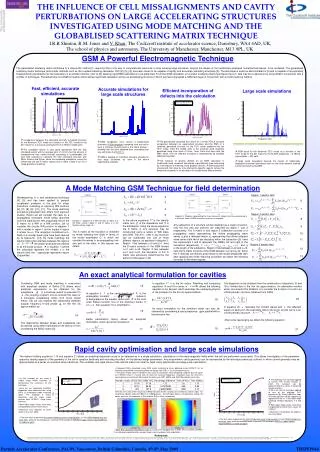
Modematching is a well established technique [4], [5] and has been applied to general accelerator problems in the past for sharp transitions consisting of adjoining WN sections [6], [7], [8], [9], [10], [11]. The mode matching procedure presented here differs from previous studies. Herein we will consider the case for a propagating monopole mode being launched form the starting port. We analytically derive the S matrix for a WN or a NW junction. Let us consider the circular WN junction in diagram 1 with n modes in region 1 and m modes in region 2 where m<=n. The analytical normalised e.m. fields in a circular beam pipe have been derived by N. Marcuvitz [12]. By mode matching the electric field at the interface between the regions i.e. we obtain what shall be referred to as the scalar product in equation 1 (where the subscripts represent the modes) is the electric field, the ^ superscript represents region IIquantities. Region 1 electric field Region 2 electric field In the above equations is the identity matrix and is the impedance and is the admittance. Using the above equations the S matrix of any structure may be constructed using a series of WN steps and GSM. The e.m... field in any structure can be subdivided into one of three different regions, as depicted in diagram 2. Region 1 lies between z=0 and z=1, here the S matrix consists of the GSM formed z=z1 and z=z3. Region 2 lies between z=z1 and z=z2, the derivation of this S matrix was previously determined by the authors of this paper in [3]. Any subsection of a structure will be classified as a region 2 section, only the first and last sections are classified as region 1 and 3 respectively. The S matrix of any region 2 subsection consists of a propagating matrix representing the infinite propagating wave series…..and a reflected matrix… representing the infinite reflected wave series both which are decaying within the subsection [3]. Here the superscripts I and II represent the GSM’s left and right of the subsection respectively, ……..………...(……………. ) and g is the length of the subsection. Region 3 lies between z=z2 and z=z3, here the S matrix consists of the GSM between z=0 and z=z2. Since the S matrices are directly proportional to the modal amplitudes then after applying the mode matching procedure we obtain the following formulae for the three regions: Region 3 electric field Combining GSM and mode matching in conjunction with analytical analysis of Bethe [13] allows exact analytical expressions to be obtained for the suseptance …..of a structure (which is equivalent to …., the coupling constant. Let us consider the case for a monopole accelerating mode; form circuit model theory [14] we can express the relationship between angular frequency and phase for the thin iris approximation as: In equation 17 is the iris radius. Rewriting and comparing equations 14 and 16 in terms of …allows the following equation to be derived, which describes the underlying physics of the problem (for the thin iris approximation). In equation 2 is the cavity length and is the propagation constant: (where b is designated as the equator radius and is the zero order Bessel function root of the dominant mode). If …………then equation 15 is simplified to: In equation 20 a represent the incident waves and b the reflected waves on each port, the subscripts refer to the ports. As this cell is in an infinite periodic structure: An exact formulation for the dominant mode can also be obtained by considering a load suseptance in parallel with a transmission line. THE INFLUENCE OF CELL MISSALIGNMENTS AND CAVITY PERTURBATIONS ON LARGE ACCELERATING STRUCTURES INVESTIGATED USING MODE MATCHING AND THE GLOBABLISED SCATTERING MATRIX TECHNIQUE I.R.R Shinton, R.M. Jones and V. Khan; The Cockcroft institute of accelerator science, Daresbury, WA4 4AD, UK; The school of physics and astronomy, The University of Manchester, Manchester, M13 9PL, UK GSM A Powerful Electromagnetic Technique The generalised scattering matrix technique is a mature RF method [1] requiring little in the way of computational resources or time allowing large structures, beyond the means of the traditionally employed numerical techniques, to be modelled. The generalised scattering matrix technique (and similar methods such as the coupled scattering calculation CSC [2], [3], [4]) has been shown to be capable of rapidly and accurately simulating structures [5]. The technique is exact as demonstrated in [5] and is capable of incorporating misalignments and defects into the calculation in an efficient manner, refer to [6], allowing rapid RMS calculations to be preformed. From the GSM calculation (or a similar scattering matrix technique) the e.m. field may be re-derived in by using GSM in conjunction with a number of techniques. Presented here is a GSM formulation which allows rapid field calculation across an accelerating structure in which we have employeed a GSM technique in conjunction with a mode matching method. Fast, efficient, accurate simulations Accurate simulations for large scale structures Efficient incorporation of defects into the calculation Large scale simulations • Comparison between the cascaded and fully simulated structure for the dominant TE11 mode as a function of the TE11 mode for the S21 matrix for a structure constructed from 3 TESLA middle cells. • The cascaded results in very good agreement with the fully simulated results with an average error of 0.014% but the amount of computational time saved through cascading is considerable; the total time required to calculate the fully simulated structure was 29hrs 25mins and 20sec, while the cascading calculation (using the referenced unit cell S matrix values) took a mere 1.5sec to run on a single processor machine. • The generalised cascaded S21 matrix for a 9-cell TESLA structure comparison between an unperturbed structure and the RMS of a randomly perturbed structure for the TE11 mode scattered into the TE11 mode. Here the middle cells in the structure were randomly perturbed using slice sizes of 0mm, 1mm, 2mm and 3mm with the RMS taken over 20 different simulations (representing 20 possible fabricated cavities). • The inclusion of realistic defects for an RMS calculation in traditionally used numerical techniques is prohibitively time consuming as it will require re-meshing of the problem domain. A GSM calculation circumvents this issue by only altering the specific regions (where the defects are located) in its calculation to include these effects directly. • GSM compilation error across a hypothetical symmetric 100m structure cascading from any cell in such a structure should result in the same answer – showing that the error obtained from cascading from any cell is less that 5x10⁻³% • . • GSM is capable of consistent accurate answers for very large structures, as seen in the above hypothetical example • GSM result for the dominant TE11 mode as a function of the TE11 mode for the S21 matrix for the FLASH accelerator – 6 TESLA cryomodules – 432 cells. • Large scale simulations beyond the means of traditionally employed numerical techniques such as the finite element method can be achieved using GSM. A Mode Matching GSM Technique for field determination 2 6 3 4 7 5 Diagram 2: Diagram representing the three classes of regions that are encountered in a structure. Here a WNW structure is used as an example. 8 Diagram 1: Diagram of a WN transition of radius b in the Wide section (region I) and of radius a in the Narrow section (region II) 9 The S matrix at the transition is obtained by mode matching the fields in terms of the modal amplitudes C, in which we consider the waves to be propagating from one port to the other, in this manner we obtain: 10 11 12 1 13 An exact analytical formulation for cavities The dispersion curve obtained from the combination of equations 15 and 18 is limited due to the thin iris approximation. An alternative method which circumvents this limitation is to consider the S matrix of a cell in an infinite periodic structure (obtained from GSM): 15 20 18 16 14 Bethe perturbation theory allows an analytical formulation, which gives the constant as: After some rearranging we obtain the following equation: The relationship between phase and suseptance can be derived using either transmission line theory or from considering the ABCD matrix [5]: 19 17 21 Rapid cavity optimisation and large scale simulations The method utilising equations 1-13 and equation 21 allows an analytical dispersion curve to be obtained as in a single calculation, calculations of the electromagnetic fields within the cell are preformed concurrently. This allows investigation of the parameter space by varying aspects of the geometry of the cell in question iteratively and recording the effect on the desired design parameters. Any axisymmetric cavity geometry can be represented by the technique previously outlined, in which curved geometry may be approximated as a series of conjoined sharp transitions. The versatility and rapid nature of the method make it an ideal for rapid cavity optimization and large scale calculations. • Compared RQ’s calculated using GSM mode matching to those obtained using HFSSv11 for an idealised sharp WNW structure based on the design from [15] i.e. a 2/3 phased structure. • The driven modal solver in HFSSv11 was used, all simulations were conducted using the discrete solver at 11.93GHz (since 1, 3 and 6 cells all share this resonant frequency), simulations were run until 0.2% convergence was achieved. Meshing for the cells were 7401, 65056 and 154215 quadratic mesh cells. • In this example we are using a simple sharp WNW transition to demonstrate the usefulness of the technique • Here we are comparing analytical dispersion curve obtained from using KN7c (a longitudinal mode matching code), The analytical S matrix calculation and the eigen mode solution from HFSSv11 using linear elements. • Note eigen mode values have been extrapolated to infinite mesh values • Maximum error between all three codes is less than 2MHz • The technique can easily be applied to cavities with curved surfaces in which the curvature can be approximated by a series of conjoined sharp transitions. • Here we see the technique applied to one of the alternate CLIC geometries [8]. Using 0.001GHz steps 30 modes per port and 50 segments to approximate the iris in the GSM mode matching method (equations 1-5 and 21) • Note eigen mode values have been extrapolated to infinite mesh values for HFSSv11 • Maximum error between the codes is less than 3MHz Here we see a slice of the results for a WNW transition for the variation of iris thickness and iris radius for a particular equator radius b=9.88mm at 120deg phase – the technique allows a full parameter sweep. The colour axes are the frequency in GHz and the R/Q in Ohms respectively • The time taken to generate the entire Dispersion curve using equation 21 (the GSM method) was less than 1min, while the meshed based numerical FEM method of HFSSv11 (eigen solver) required 30mins or mode per point! • The time taken to generate the entire Dispersion curve using equation 21 (the GSM method) was less than 1min, while the meshed based numerical FEM method of HFSSv11 (eigen solver) required 45mins or mode per point! • Each R/Q calculation required less than 1s (using a PC equipped with a 3GHz CPU and 4GHz of RAM ) – thus allowing large parameter sweeps/ large scale simulations to be undertaken References [1] I.R.R. Shinton and R.M. Jones, PAC, 2007, p2218; [2] I.R.R. Shinton and R.M. Jones, 13th International workshop on RF Superconductivity, 2007, WEP80; [3] I.R.R. Shinton and R.M. Jones, EPAC, 2008, p619; [4] R.E. Collin, Foundations for microwave engineering,1966; [5] R.E. Collin, Field theory of guided waves, 1991 ; [6] U.van. Rienen, AIP Conf. Proc, 1997, Vol 391, p89; [7] S.A. Heifets and S.A. Kheifets, SLAC-PUB-5907; [8] S.A. Heifets and S.A. Kheifets, SLAC-PUB-5562; [9] V.A.Dolgashev, ICAP, 1998, p149; [10] V.Dolgashev, T.Higo,Proceedings of the 8th international workshop on linear colliders, LC97,1997.; [11] L. Carin, Computational analysis of cascaded coaxial and circular waveguide discontinuities, Masters thesis, University of Maryland, 1986, 12] N.Marcuvitz, The wave guide handbook, 1986; [13] H. Henke, TET-Note 96/04, August 1996; [14] K.L.F. Bane SLAC-PUB-5783; [15] L.F. Wang, Y.Z. Lin, T.Higo and K. Takata, PAC, 2001, pg 3045; [15] R.M.Jones and V.F.Khan, LINAC08, 2008, MOP105 Particle Accelerator Conference, PAC09, Vancouver, British Columbia, Canada, 4th-8th May 2009 TH5PFP044