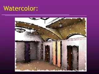
Computer Generated Watercolor
Computer Generated Watercolor. Curtis, Anderson, Seims, Fleisher, Salesin SIGGRAPH 1997. Presented by Yann SEMET Universite of Illinois at Urbana Champaign Universite de Technologie de Compiegne. Background. NPR Purpose : aesthetic rather than technical Artificial art ?.

Computer Generated Watercolor
E N D
Presentation Transcript
Computer Generated Watercolor Curtis, Anderson, Seims, Fleisher, Salesin SIGGRAPH 1997 Presented by Yann SEMET Universite of Illinois at Urbana Champaign Universite de Technologie de Compiegne
Background • NPR • Purpose : aesthetic rather than technical • Artificial art ?
Overview • Particularities of Watercolor • Computer simulation • Fluid simulation • Kubelka-Munk rendering • Applications • Discussion
Like no other medium • Beautiful textures and patterns • Reveals the motion of water • Luminous, glowing
Watercolor materials • Paper • Pigments
Dry brush Edge darkening Back runs Granulation Flow Glazing Watercolor effects
Fluid simulation I • 3 layers :
Fluid simulation II • Parameters of the simulation : • Wet-area mask : M • Velocities : u,v • Pressure : p • Concentration : gk • Height of paper : h • Physical properties : density, staining power, granularity, etc. • Fluid properties : saturation, capacity, etc.
Paper simulation • Supposedly : shape of every fiber matters • A simpler model : a height field • Generation : Perlin’s noise and Worley’s cellular textures
Main loop • For each time step • Move Water • Update velocities • Relax Divergence • Flow Outward • Move Pigment • Transfer Pigment • Simulate Capillary Flow
Conditions for realism • Flow must be constrained so water remains within M • Surplus of water causes flow outward • Flow must be damped to minimize oscillating waves • Flow is perturbed by texture of paper • Local changes have global effects • Outward flow to darken edges
Rendering : Kubelka-Munk • For each pigment, 2 coeff. Per RGB layer : • K : absorbtion • S : scattering • Supposedly : K and S are measured • Here : user provides Rw and Rb
Types of paints • Opaque (e.g. Indian Red) • Transparent (e.g. Quinacridone Rose) • Interference (e.g. Interference Lilac) • Different hues (e.g. Hansa Yellow)
Optical compositing • Compute R and T : • Then compose : • Weight relatively to relative thicknesses
Discussion of the KM model • Assumptions partially satisfied : • Identical refractive indices • Random orientation of pigments • Diffuse illumination • 1 wavelength at a time • No chemical interaction • Works surprisingly well ! • OK, because we’re looking for appearance, not actual modeling
Application I • Interactive painting :
Application II • Watercolorization :
Application III • 3D models :
Future work • Other effects • Automatic rendering • Generalization • Animation
Summary • A particular painting technique • A physically based simulation • Fluid motion • Optical compositing • Application and results
Conclusion and discussion • Efficiency issues and long term interest • Border between art, physics and computer science