Download
1 / 26
260 likes | 517 Vues
Hierarchical Semantic Indexing for Large Scale Image Retrieval. Jia Deng(Princeton University) Alexander C. Berg(Stony Brook University) Li Fei-Fei (Stanford University). Outline. Introduction Exploiting Hierarchy for Retrieval Efficient Indexing Experiments Conclusion. Introduction.

E N D
Hierarchical Semantic Indexing for Large Scale Image Retrieval Jia Deng(Princeton University) Alexander C. Berg(Stony Brook University) Li Fei-Fei(Stanford University)
Outline • Introduction • Exploiting Hierarchy for Retrieval • Efficient Indexing • Experiments • Conclusion
Introduction • Prior knowledge: • Known semantic labels and a hierarchy relation relating them • Contributions: • Exploiting retrieval with semantic hierarchically • Novel hashing scheme
Low-lv Features to semantic vector • Using method of : Beyond Bags of Features: Spatial Pyramid Matching for Recognizing Natural Scene Categories[24] (SPM)
Low-lv Features to semantic vector • Classification is done with SVM trained using the one-versus-all rule: • a classifier is learned to separate each class from the rest, and the test image is assigned the label of the classifier with the highest response. • Train linear SVM with semantic attributes by LIBLINEAR • 2-fold cross validation to determine C parameter
Hard Assign / Probability Calibration • Hard Assign : • δi(a) ∈ {0,1} , image a has attribute i or not • Example : image a is a person δperson(a) = 1 • xi=δi • The binary entry here called “hard assign” • Probability Calibration • Fit sigmoid function to SVM classifier to get prob. • xi=Pr(δi(a)=1|a) , prob. of image a has attribute i
Hierarchy • Let Sij = ξ(π(i,j)) , similarity between attributes • π(i,j) is lowest common ancestor of attribute i and j • ξ : {1,..,K}=> R , similarity function (We can assign scores base on height of node) Example: • In experiment, define ξ=1-h(π(i,j))/h* h* is total height of node Equine Donkey Horse
Flat • When attributes are mutually exclusive • No hierarchical relationship between relationships • This is the most existing system developed and evaluated • Equivalent to setting S matrix to identity
Similarity • Similarity between image a and b is ∑ijδi(a)Sijδj(b) , S ∈RKxK,S is matching score between attribute i and j,K is number of attributes (like vector multiplication xTSy, author refer this as bilinear similarity) *Cosine Similarity is
Multinomial Distribution • Suppose • P(蝦) = 0.2 • P(蟹) = 0.35 • P(魚) = 0.45 • P(N蝦= 8, N蟹= 10, N魚= 12) • = (0.2)8(0.35)10(0.45)12
Sampling • For each trial, draw an auxiliary variable X from a uniform (0, 1) distribution. The resulting outcome is the component • This is a sample for the multinomial distribution with n = 1
Hashing • Prior condition: • S is symmetric • S is element-wise non-negative • S is diagonally dominant, i.e.
Hashing • Define a K × (K + 1) matrix Θ : Θij(i,j ≤K) • Each row of Θ sums to one, and Θ without last column is symmetric
Hashing • Consider hash functions of the form h outputs a subset in 2N, • 2N is all subsets of natural numbers. • h(x) = h(y) is defined as “set equality”, that is {a,b,c} = {b,a,c}
Hashing • To construct H(S,ε), let N ≥ 1/ ε, Then h(x; S, ε) is computed as follows: • (1) Sample α ∈ {1, . . . , K} ∼multi(x) • (2) Sample β ∈ {1, . . . , K + 1} ∼ multi(θα) where θαis the αth row of Θ; • (3) If β ≤ K, return {α, β}; • (4) Randomly pick γ from {K+1, . . . , K+N} and return {γ}.
Experiments • Used Datasets: • Caltech 256 • ILSVRC (for precision evaluation) • (half for train, half for test) • 21k dimensional vectors formed by three-level SPM on published SIFT visual words from 1000 word codebook • Train linear SVM with semantic attributes by LIBLINEAR, 2-fold cross validation for C
Precision • Suppose we have retrieved 2 images with similarity 0.8 and 0.7, but ground truth is 5 images with similarity {0.8,0.7,0.6,0.5,0.4} • Ordinary Precision : 2/5 = 0.4 • Proposed Precision : (0.8+0.7)/(0.8+0.7+0.6+0.5+0.4) = 0.5
Precision Definition • Precision measure for a query q • Numerator(分子) : sum of ground truth similarities for most similar k database items • Denominator(分母): sum of ground truth similarities for the best possible k database items
Conclusion • Present an approach that can exploit prior knowledge of a semantic hierarchy for similar image retrieval • Outperform state-of-art similarity learning (OASIS) with more accuracy and less computation • A hashing scheme for bilinear similarity on probability distributions
End Thank You