Chapter 5 Finite-Length Discrete Transforms

1. Chapter 5 Finite-Length Discrete Transforms Definition of DFT The Relationship Between DFT and DTFT DFT Properties DFT Computation FFT

2. 5.1 Orthogonal Transforms • General form of the orthogonal transform pair: analysis equation synthesis equation • ψ[k,n] called the basis sequences, are also length-N sequences in both domains, which satisfy:

3. 5.2 Discrete Fourier Transform (DFT) Time domain Frequency domain Continuous Aperiodical FT Continue Aperiodical Continuous Periodical  FS  Discrete Aperiodical Discrete Aperiodical DTFT Periodical Continuous Discrete & Periodical  DFS  Periodical & Discrete

4. ω0 = 2π/T ω0δω0(ω) δT(t)  -2ω0 - ω0 0 ω0 2ω0 ω -2T -T 0 T 2T t Typical DFT Pair • δT(t)  ω0δω0(ω) • The signals in both sides are periodical, so the processing could be in one period, which is important because (1) the number of calculation is limited, which is necessary for computer; (2) all of the signal information could be kept in one period, which is necessary for accurate processing.

5. Make a Signal Discrete and Periodical • The engineering signals are often continuous and aperiodical. If we want to process the signals with DFT, we have to make the signals discrete and periodical. • Sampling to make the signal be discrete. • Make the signal periodical by periodical expanding. • If x[n] is a limited length N-point sequence, see it as one period of a periodical signal; • If x[n] is an infinite length sequence, cut-off its tail to make a N-point sequence, then do the periodic extending. The truncation will introduce distortion. ---- windowing

6. Make a signal discrete and periodical

7. 2 1 3 4 Re[z] k=0 7(k=N-1) 5 6 From DTFT to get DFT • DTFT: discrete in time domain, continuous in frequency domain. • Sampling the DTFT of sequences to get N frequency points to research, that is DFT.

8. 5.2.1 The Definition of DFT Where: Which can easily be deduced from:

9. The Definition of DFT • Note: X[k] is also a length-N sequence in the frequency domain. • The sequence X[k] is called the Discrete Fourier Transform (DFT) of the sequence x[n]. • To verify the above expression we multiply both sides of the above equation by WNln and sum the result from n = 0 to n=N-1.

10. resulting in: Hence,

11. The Definition of DFT • Example - Consider the length-N sequence: Its N-point DFT is given by:

12. The Definition of DFT • Example - Consider the length-N sequence: Its N-point DFT is given by:

13. The Definition of DFT • Example - Consider the length-N sequence defined for 0 ≤n ≤N-1 • Using a trigonometric identity we can write:

14. The Definition of DFT The N-point DFT of g[n] is thus given by:

15. r an integer The Definition of DFT Making use of the identity: we get:

17. 5.2.2 Matrix Relations • The DFT samples defined by: Can be expressed in matrix form as X=DNx Where X=[x[0] x[1] … X[N-1]]T x=[x[0] x[1] … x[N-1]]T

18. Matrix Relations • And DN is the NN DFT matrix given by:

19. Matrix Relations • Likewise, the IDFT relation given by: can be expressed in matrix form as x=DN-1X, where DN-1 is the NN IDFT matrix.

20. Matrix Relations Note: DN-1 = (DN*) / N

21. 5.2.3 DFT Computation Using MATLAB • The functions to compute the DFT and the IDFT are FFTandIFFT. • These functions make use of FFT algorithms which are computationally highly efficient compared to the direct computation. • From O(n2) to O(nlog2n) • Programs 5_1.mand 5_2.millustrate the use of these functions.

22. indicates DFT samples • Example - Program 5_3.m can be used to compute the DFT and the DTFT of the sequence: • fft(x, N) • N=16

23. fft(x, 80)

24. fft(x, 20)

25. 5.3 Relation Between the DTFT and the DFT and the Their Inverses • The relation between the DTFT and the N-point DFT of a length-N sequence. • Numerical computation of the DTFT using the DFT. • DTFT from DFT by interpolation. • Sampling the DTFT.

26. 5.3.1 Relation with DTFT • DTFT: discrete in time domain, continuous in frequency domain. • Sampling the DTFT of sequences with the space is 2π/N to get N frequency points, that is DFT.

27. 5.3.2 Numerical Computation of the DTFT Using the DFT How to compute the DTFT of a length-N sequence x[n] by using computer? 1.Sampling the X(ejw)to get a length-M sequence, M>>N. Each frequency component is X(ej2π/M). 2.If the DFT of a sequence is length-M, the sequence must be a length-M sequence. So we build a length-M sequence use x[n]. • The function freqz employs this approach to evaluate the frequency response at a prescribed set of frequencies of a DTFT expressed as a rational function in e-jω.

28. We can see above equation is the DFT of a length-M sequence. Because M>>N, it can be seen as an approach of the DTFT of a length-N sequence.

29. 5.3.3 DTFT from DFT by Interpolation • The N-point DFT X[k] of a length-N sequence x[n] is simply the frequency samples of its DTFT X(ejω) evaluated at N uniformly spaced frequency points ω=ωk=2πk/N, 0≤k≤N-1. • Given the N-point DFT X[k] of a length-N sequence x[n], its DTFT X(ejω) can be uniquely determined from X[k].

30. DTFT from DFT by Interpolation Thus:

31. DTFT from DFT by Interpolation • To develop a compact expression for the sum S,

32. DTFT from DFT by Interpolation • Therefore: X(ejω) is interpolated.

33. 5.3.4 Sampling the DTFT • Consider a sequence x[n] with DTFT X(ejω). • We sample X(ejω) at N equally spaced points ωk=2πk/N, 0≤k≤N-1 developing the N frequency samples {X(ejωk)}. • These N frequency samples can be considered as an N-point DFT Y[k] whose N-point IDFT is a length-N sequence y[n].

34. Sampling the DTFT Now Thus: An IDFT of Y[k] yields:

35. Sampling the DTFT Making use of the identity:

36. Sampling the DTFT • We arrive at the desired relation: Thus y[n] is obtained from x[n] by adding an infinite number of shifted replicas of x[n], with each replica shifted by an integer multiple of N sampling instants, and observing the sum only for the interval 0≤n≤N-1.

37. Sampling the DTFT • To apply： to finite-length sequences, we assume that the samples outside the specified range are zeros. Thus if x[n] is a length-M sequence with M≤N, then y[n]=x[n] for 0≤n≤N-1.

38. Sampling the DTFT • If M>N, there is a time-domain aliasing of samples of x[n] in generating y[n], and x[n] cannot be recovered from y[n]. • Example: Let {x[n]}={0 1 2 3 4 5} ↑ By sampling its DTFT X(ejω) at ωk=2πk/4, 0≤k≤3 and then applying a 4-point IDFT to these samples, we arrive at the sequence y[n] given by:

39. Sampling the DTFT • i.e. {y[n]}={4 6 2 3} ↑ {x[n]} cannot be recovered from {y[n]}

41. 5.4 Operations on Finite-Length Sequences • The DFT properties also show useful functions in signal processing applications. • Two operations: (1) Circular Shift of a Sequence (2) Circular Convolution

42. 5.4.1 Circular Shift of a Sequence • Consider length-N sequences defined for 0≤n≤N-1, Sample values of such sequences are equal to zero for values of n < 0 and n≥N. • For any arbitrary integer n0 , the shifted sequence x1[n] = x[n – n0] is no longer defined for the range 0≤n≤N-1. • We thus need to define another type of a shift that will always keep the shifted sequence in the range 0≤n≤N-1. ----Circular Shift of length-N sequence x[n]: xc[n]=x[<n-n0>N]

43. Circular Shift of length-N sequence x[n]: • There are two ways to perform Circular Shift: (1) Using the “modulo” operation; (2) Period expand.

44. Circular Shift of a Sequence Illustration of the concept of a circular shift:

45. x[n] x[n-1] Circular Shift of a Sequence Non-circular shift circular shift

46. N N = g[n] h[n] = g[n] h[n] 5.4.2 Circular convolution • To develop a convolution-like operation resulting in a length-N sequence yC[n], we need to define a circular time-reversal, and then apply a circular time-shift. • Circular convolution defined as:

47. The N-point circular convolution can be written in matrix form as: • Note: The elements of each diagonal of the NN matrix are equal • Such a matrix is called a circulant matrix

48. 4 n n • Example - Determine the 4-point circular convolution of the two length-4 sequences: as sketched below: • The result is a length-4 sequence yC[n] given by:

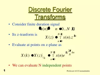
49. g[k] g[k] g[k] g[k] g[k] h[k] h[1-k] h[2-k] h[3-k] h[-k] y[2] y[3] y[0] y[1] 7 6 6 5 g[n] =δ[n] +2δ[n-1] +δ[n-3] h[n] = 2δ[n] +2δ[n-1] +δ[n-2] +δ[n-3] y[n]=6δ[n]+7δ[n-1]+6δ[n-2]+5δ[n-3]

50. From the above we observe: