Download
1 / 28
290 likes | 392 Vues
Utilizing GIS and statistical models to predict groundfish and cetacean abundance based on environmental variables and spatial autocorrelation. Assessing errors to understand marine ecology. Incorporates NOAA data and advanced modeling techniques for accurate predictions.

E N D
Extending GIS with Statistical Modelsto Predict Marine Species Distributions Zach Hecht-Leavitt NY Department of State Division of Coastal Resources
Offshore Planning NY Long Island NJ
Goals • Predict the abundance of selected groundfish species as a function of: • environmental/habitat variables • spatial autocorrelation • Assess error • Understand ecology
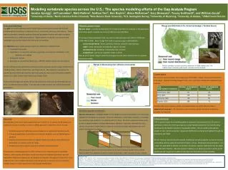
The Fish Data • NOAA Northeast Fisheries Science Center bottom trawl (catches groundfish) • Biannual 1975-2009 • Standardized gear, speed, and distance • Cleaned by Stone Environmental • Break down by season and life stage • 6 species selected NOAA NEFSC NOAA NEFSC
The Environmental Data • Depth • Distance from Shelf Edge • Bottom Grain Size • Slope • Sea Surface Temperature* • Chlorophyll* • Stratification* • Turbidity* • Zooplankton* • Provided by NOAA Biogeography Branch *Long-term, seasonal average
Data Exploration Adult Fluke Count • Approximate environmental relationships with lineartrend • Data is extremelyskewed (lots of zeroes) • Go with Zero-Inflated Generalized Linear Models (GLMs)
Workflow • “Loose” coupling • With 10.x can “hard” couple via Geospatial Modeling Environment (GME) Y=B1X1+B2X2… .CSV zeroinfl(), AchimZeileis
Workflow = + B2 * B1* B3 * +
The Residual -3 +5 -9 -1 +2 +3 +4 +1 -4 +2
Modeling Steps = + Predictors (GLM) + Residual (kriging) = Mean Expectation + Error (unexplained variation)
Error Assessment -4 +2 -1 -3 +2 +3
Error Assessment • 50/50 cross-validation • Smooth error with moving window • Final maps based on full dataset • Conservative error estimates
Final product (fluke example) M L L H L
Goals • Predict the abundance of selected groundfish as a function of: • environmental/habitat variables • spatial autocorrelation • Assess error • Understand ecology
Another Approach to Dealing with Zeroes
Another Approach • Rather than a one-size-fits all model… • … model presence/absence and abundance with two separate stages • May better reflect ecological reality • More conservative approach
Goals • Predict the abundance of selected cetaceans as a function of: • spatial autocorrelation • Assess error
The Marine Mammal Data • North Atlantic Right Whale Consortium Database • Aerial and shipboard surveys, 1978 - 2009 • Cleaned by New England Aquarium • SPUE • 4 species/groups selected • No predictors this time! NOAA SWFSC NOAA SWFSC
Stage I – Presence/Absence 1 1 4 1 1 5 1 2 1 0 0 0 1 1 1 1 1 1 3 4 1 1 4 1 2 0 0 0 3 1 0 0 0 0 0 0 0 4 2 0 0 0 0 1 1 0 0 0
Stage I – Presence/Absence 1 1 1 0 1 1 1 0 0 0 ROC Curve Epi package, Carstensen et. al.
Goals • Predict the abundance of selected cetaceans as a function of: • spatial autocorrelation • Assess error
Further reading • Hengl, T., G.B.M. Heuvelink and D.G. Rossiter. 2007. About regression-kriging: From equations to case studies. Computers and Geosciences 33:1301-1315. • Wenger, S. J. and M. C. Freeman. 2008. Estimating Species Occurrence, Abundance, And Detection Probability Using Zero-Inflated Distributions. Ecology 89:2953-2959 • Monestiez, P., L. Dubroca, E. Bonnin, J.-P. Durbec, C. Guinet. 2006. Geostatistical modeling of spatial distribution of Balaenopteraphysalus in the Northwestern Mediterranean Sea from sparse count data and heterogeneous observation efforts. Ecological Modeling, 193: 615-628. • Menza, C., B.P. Kinlan, D.S. Dorfman, M. Poti and C. Caldow (eds.). 2012. A Biogeographic Assessment of Seabirds, Deep Sea Corals and Ocean Habitats of the New York Bight: Science to Support Offshore Spatial Planning. NOAA Technical Memorandum NOS NCCOS 141. Silver Spring, MD. 224 pp.
Thank you! Zach.Hecht-Leavitt@dos.ny.gov / zhechtle@gmail.com