Optical illusion ? Correlation ( r or R or )
510 likes | 649 Vues
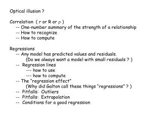
Optical illusion ? Correlation ( r or R or ) -- One-number summary of the strength of a relationship -- How to recognize -- How to compute Regressions -- Any model has predicted values and residuals. (Do we always want a model with small residuals ? ) -- Regression lines

Optical illusion ? Correlation ( r or R or )
E N D
Presentation Transcript
Optical illusion ? • Correlation ( r or R or ) • -- One-number summary of the strength of a relationship • -- How to recognize • -- How to compute • Regressions • -- Any model has predicted values and residuals. • (Do we always want a model with small residuals ? ) • -- Regression lines • --- how to use • --- how to compute • -- The “regression effect” • (Why did Galton call these things “regressions” ? ) • -- Pitfalls: Outliers • -- Pitfalls: Extrapolation • -- Conditions for a good regression
Kinds of Association… • Positive vs. Negative • Strong vs. Weak • Linear vs. Non-linear
CORRELATION • CORRELATION • (or, the CORRELATION COEFFICIENT) • measures the strength of a linear relationship. • If the relationship is non-linear, it measures the strength of the linear part of the relationship. But then it doesn’t tell the whole story. • Correlation can be positive or negative.
correlation = .97 correlation = .71
2 2 1 1 0 0 Y Y -1 -1 -1 0 1 2 -2 0 2 X X correlation = –.97 correlation = –.71
2 1 0 Y -1 -1 0 1 2 X correlation = .97 correlation = .97
correlation = .24 correlation = .90
correlation = .50 correlation = 0
Computing correlation… • Replace each variable with its standardized version. • Take an “average” of ( xi’ times yi’ ):
Computing correlation sum of all the products r, or R, or greek (rho) n-1 or n ?
Good things about correlation • It’s symmetric ( correlation of x and y means same as correlation of y and x ) • It doesn’t depend on scale or units • — adding or multiplying either variable by • a constant doesn’t change r • — of course not; r depend only on the • standardized versions • r is always in the range from -1 to +1 • +1 means perfect positive correlation; dots on line • -1 means perfect negative correlation; dots on line • 0 means no relationship, OR no linear relationship
Bad things about correlation • Sensitive to outliers • Misses non-linear relationships • Doesn’t imply causality
Made-up Examples STATE AVE SCORE PERCENT TAKING SAT
Made-up Examples IQ SHOE SIZE
Made-up Examples JUDGE’S IMPRESSION 450 250 350 BAKING TEMP
Made-up Examples LIFE EXPECTANCY GDP PER CAPITA
Observed Values, Predictions, and Residuals resp. var. explanatory variable
Observed Values, Predictions, and Residuals resp. var. explanatory variable
Observed Values, Predictions, and Residuals resp. var. explanatory variable
Observed Values, Predictions, and Residuals Observed value Predicted value resp. var. Residual = observed – predicted explanatory variable
Linear models and non-linear models • Model A: Model B: • y = a + bx + error y = a x1/2 + error • Model B has smaller errors. Is it a better model?
aa opas asl poasie ;aaslkf 4-9043578 • y = 453209)_(*_n &*^(*LKH l;j;)(*&)(*& + error • This model has even smaller errors. In fact, zero errors. • Tradeoff: Small errors vs. complexity. • (We’ll only consider linear models.)
About Lines • y = mx + b slope = m b
About Lines • y = mx + b slope = m y intercept b slope
About Lines • y = mx + b slope = m b
About Lines • y = mx + b • y = b + mx slope = m b
About Lines • y = mx + b • y = b + mx • y = + x • y = 0 + 1x
About Lines • y = mx + b • y = b + mx • y = + x • y = 0 + 1x • y = b0 + b1x
About Lines • y = mx + b • y = b + mx • y = + x • y = 0 + 1x • y = b0 + b1x slope = b1 b0 slope y intercept
About Lines • y = mx + b • y = b + mx • y = + x • y = 0 + 1x • y = b0 + b1x slope = b1 b0 slope y intercept
Computing the best-fit line • In STANDARDIZED scatterplot: • -- goes through origin • -- slope is r • In ORIGINAL scatterplot: • -- goes through “point of means” • -- slope is r × Y x
The “Regression” Effect • A preschool program attempts to boost children’s reading scores. • Children are given a pre-test and a post-test. • Pre-test: mean score ≈ 100, SD ≈ 10 • Post-test: mean score ≈ 100, SD ≈ 10 • The program seems to have no effect.
A closer look at the data shows a surprising result: • Children who were below average on the pre-test tended to gain about 5-10 points on the post-test • Children who were above average on the pre-test tended to lose about 5-10 points on the post-test.
A closer look at the data shows a surprising result: • Children who were below average on the pre-test tended to gain about 5-10 points on the post-test • Children who were above average on the pre-test tended to lose about 5-10 points on the post-test. • Maybe we should provide the program only for children whose pre-test scores are below average?
Fact: • In most test–retest and analogous situations, the bottom group on the first test will on average tend to improve, while the top group on the first test will on average tend to do worse. • Other examples: • • Students who score high on the midterm tend on average to score high on the final, but not as high. • • An athlete who has a good rookie year tends to slump in his or her second year. (“Sophomore jinx”, "Sports Illustrated Jinx") • • Tall fathers tend to have sons who are tall, but not as tall. (Galton’s original example!)
It works the other way, too: • • Students who score high on the final tend to have scored high on the midterm, but not as high. • • Tall sons tend to have fathers who are tall, but not as tall. • • Students who did well on the post-test showed improvements, on average, of 5-10 points, while students who did poorly on the post-test dropped an average of 5-10 points.
Students can do well on the pretest… • -- because they are good readers, or • -- because they get lucky. • The good readers, on average, do exactly as well on the post-test. The lucky group, on average, score lower. • Students can get unlucky, too, but fewer of that group are among the high-scorers on the pre-test. • So the top group on the pre-test, on average, tends to score a little lower on the post-test.
Extrapolation • Interpolation: Using a model to estimate Y • for an X value within the range on which the model was based. • Extrapolation: Estimating based on an X value outside the range.
Extrapolation • Interpolation: Using a model to estimate Y • for an X value within the range on which the model was based. • Extrapolation: Estimating based on an X value outside the range. • Interpolation Good, Extrapolation Bad.
Nixon’s Graph:Economic Growth Start of Nixon Adm.
Nixon’s Graph:Economic Growth Start of Nixon Adm. Now
Nixon’s Graph:Economic Growth Start of Nixon Adm. Projection Now
Conditions for regression • “Straight enough” condition (linearity) • Errors are mostly independent of X • Errors are mostly independent of anything else you can think of • Errors are more-or-less normally distributed