Download
1 / 37
370 likes | 589 Vues
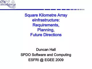
Square Kilometre Array Computational Challenges Paul Alexander. What is the Square Kilometre Array (SKA). Next Generation radio telescope – compared to best current instruments it is ... ~100 times sensitivity ~ 10 6 times faster imaging the sky

E N D
Square Kilometre ArrayComputational ChallengesPaul Alexander
What is the Square Kilometre Array (SKA) • Next Generation radio telescope – compared to best current instruments it is ... • ~100 times sensitivity • ~ 106 times faster imagingthe sky • More than 5 square km ofcollecting area on sizes3000km E-MERLIN eVLA 27 27m dishes Longest baseline 30km GMRT 30 45m dishes Longest baseline 35 km
What is the Square Kilometre Array (SKA) • Next Generation radio telescope – compared to best current instruments it is ... • ~100 times sensitivity • ~ 106 times faster imaging the sky • More than 5 square km of collecting area on sizes3000km • Will address some of the key problems of astrophysics and cosmology (and physics) • Builds on techniques developed in Cambridge • It is an interferometer • Uses innovative technologies... • Major ICT project • Need performance at low unit cost
also a Continental sized Radio Telescope • Need a radio-quiet site • Very low population density • Large amount of space • Possible sites (decision 2012) • Western Australia • Karoo Desert RSA
Sensitivity comparison SKA2 SKA1 EVLA LOFAR
SKA2 ~ 250 Dense Aperture Array Stations 300-1400MHz ~ 2700 Dishes 3-Core Central Region Wide Band Single Pixel Feeds ~250 Sparse Aperture Array Stations 70-450MHz Phased Array Feeds800 MHz – 2GHz Artist renditions from Swinburne Astronomy Productions
SKA1 ~ 300 Dishes 2-Core Central Region Wide Band Single Pixel Feeds ~50 Sparse Aperture Array Stations 70-450MHz Artist renditions from Swinburne Astronomy Productions
SKA Timeline • 2019Operations SKA1 2024: Operations SKA2 • 2019-2023 Construction of Full SKA, SKA2€1.5B • 2016-201910% SKA construction, SKA1€300M • 2012 Site selection • 2012 - 2016Pre-Construction: 1 yr Detailed design€90M • PEP 3 yrProduction Readiness • 2008 - 2012System design and refinement of specification • 2000 - 2007Initial concepts stage • 1995 - 2000Preliminary ideas and R&D
Work Packages in the PEP Management System Science Maintenance and support /Operations Plan Site preparation Dishes Aperture arrays Signal transport & networks Signal processing Science data processor Telescope manager Power SPO Work Package Contractors
Work Packages in the PEP Management System Science Maintenance and support /Operations Plan Site preparation Dishes Aperture arrays Signal transport & networks Signal processing Science data processor Telescope manager Power SPO Work Package Contractors UK (lead), AU (CSIRO…), NL (ASTRON…) South Africa SKA, Industry (Intel, IBM…)
Standard interferometer s Astronomical signal (EM wave) • Visibility: • V(B) = E1 E2* • = I(s) exp( iwB.s/c ) • Resolution determined by maximum baseline • qmax ~ l / Bmax • Field of View (FoV) determined by the size of each dish • qdish ~ l / D B . s Detect & amplify B 1 2 Digitise & delay Correlate X X X X X X Integrate visibilities SKY Image Process Calibrate, grid, FFT
Aperture arrays Digitise, delay & beam form • Beam form: • Apply delay gradients to point electrically • Multiple delay gradients • many beams and large FoV Correlate X X X X X X SKY Image Process Calibrate, grid, FFT
Aperture arrays • Aperture-Array station • ~25000 phased elements • Equivalent to one dish • These are then cross-correlated Digitise, delay & beam form • Beam form: • Apply delay gradients to point electrically • Multiple delay gradients • many beams and large FoV Correlate X X X X X X SKY Image Process Calibrate, grid, FFT
Formulation • What we measure from a pair of telescopes: • In practice we have to deal with this equation, butfor simplicity consider a scalar model m l • The delays allow us to follow a point on the sky • The Ji are direction dependent Jones matrices which include the effects of: • propagation from the sky through the atmosphere • scattering • coupling to the antenna/detector • gain s
Formulation • Where we include time delays to follow a central point. In terms of direction cosines relative to the point we follow and for a b = (u,v,w) • If we can calibrate our system we can apply our telescope-dependent calibrations and then for small FoV we can approximate • And the measured data are just samples of this function • In this case we can estimate the sky viaFourier inversion and deconvolution m l s
Formulation • Sampling of the Fourier plane is determined by the positioning of the antennas and improved by the rotation of the earth m l We s
SKA Key Science Drivers ORIGINS • Neutral hydrogen in the universe from the Epoch of Re-ionisationto now • When did the first stars and galaxies form? • How did galaxies evolve?Role of Active Galactic Nuclei • Dark Energy, Dark Matter • Cradle of Life FUNDAMENTAL FORCES • Pulsars, General Relativity & gravitational waves • Origin & evolution of cosmic magnetism TRANSIENTS (NEW PHENOMENA) Science with the Square Kilometre Array (2004, eds. C. Carilli & S. Rawlings, New Astron. Rev., 48)
Galaxy Evolution back to z~10? HDF VLA ~ 3000 galaxies ~15 radio sources
Galaxy Evolution back to z~10? HDF SKA
The Imaging Challenge • This illustrates one of our main challenges • To make effective use of the improved sensitivity we face an immediate problem • Typically within the field of view of the telescope the noise level will be ~106 – 107 times less than the peak brightness • We have to achieve sufficiently good calibration and image fidelity to routinely achieve a “dyanamic range” of > 107:1 • With very hard work now we can just get to 106:1 in some fields
SKA2 wide area data flow 20 Gb/s 4Pb/s 16 Tb/s 24Tb/s 20 Gb/s
SKA1 Data rates from receptors • Dishes • Depends on feeds, but illustrate by 2 GHz bandwidth at 8-bits • G = 64 Gb/s from each dish • For Phased Array feeds increased by number of beams (~20) • G ~ 1 Tb/s • For Low frequency Aperture Arrays : • Bandwidth is 380 MHz • Driven by the requirements of Field of View from the science requirements which from DRM is 5 sq-degrees 20 beams • G = 240 Gb/s • These are from each collector into the correlator or beam former • 300 dishes • 285 75-m AA stations • G(total) ~ 68 Tb/s
Data Rates • After correlation the data rate is fixed by straightforward considerations • Must sample fast enough (limit on integration time) dt • Baseline B/l • UV (Fourier) cell size D/l • Must have small-enough channelwidth to avoid chromatic aberration maxB/l– B/(l+dl) maxWdt
Data rates from the correlator Standard results for integration/dump time and channel width Data rate then given by # antennas # polarizations # beams word-length Can reduce this using baseline-dependent integration times and channel widths
Example correlator data rates and products SKA1 • Aperture Array Line experiment (e.g. EoR) • 5sq degrees; 170000 channels over 250 MHz bandwidth • ~ 30 GB/s reducing quickly to ~ 1GB/s • Up to 500 TB UV (Fourier) data; Images (3D) ~ 1.5 TB • Continuum experiment with long baselines with the AA • 100 km baseline with the low-frequency AA • 1.2 TB/s reducing to ~ 12.5 GB/s • Up to 250 TB/day to archive if we archive raw UV data • Spectral-line imaging with dishes • Data rates ~ 50 GB/s; Images (3D) ~ 27 TB
Example beam-formed data rates SKA1 • Pulsar search • Galactic-plane survey for pulsars • ~ 400 GB/s to de-disperser (hardware?) • Data products are of small volume as all analysis is done in pseudo real-time.
Data Products • ~0.5 – 10 PB/day of image data • Source count ~106 sources per square degree • ~1010 sources in the accessible SKA sky, 104 numbers/record • ~1 PB for the catalogued data 100 Pbytes – 3 EBytes / year of fully processed data
The SKA Processing Challenge Correlator Visibility processors Image formation Science analysis, user interface & archive switch AA: 250 x 16 Tb/s Dish: 3000 x 60 Gb/s ~ 200 Pflop to 2.5 Eflop ~10-100 PFlop ~ ? PFlop ~1 – 500 Tb/s Software complexity
Conclusions • The next generation radio telescopes offer the possibility of transformational science, but at a cost • A major processing challenge • Need to analyse very large amounts of streaming data • Current algorithms iterative – need to buffer data • Problem too large to, for example, use a direct Bayesian approach • Are our (approximate) algorithms good enough to take into account all error effects that need to be modelled? • Only recently have we had to consider most of the effects – what have we forgotten? • Phased approach to SKA is very good for the processing – performance increasing and critically we can continually learn