Unsupervised Learning

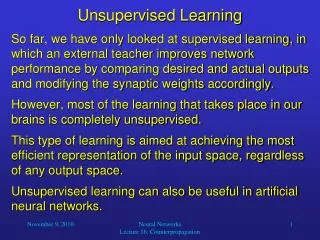
Unsupervised Learning • So far, we have only looked at supervised learning, in which an external teacher improves network performance by comparing desired and actual outputs and modifying the synaptic weights accordingly. • However, most of the learning that takes place in our brains is completely unsupervised. • This type of learning is aimed at achieving the most efficient representation of the input space, regardless of any output space. • Unsupervised learning can also be useful in artificial neural networks. Neural Networks Lecture 16: Counterpropagation

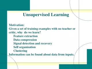
Unsupervised Learning • Applications of unsupervised learning include • Clustering • Vector quantization • Data compression • Feature extraction • Unsupervised learning methods can also be combined with supervised ones to enable learning through input-output pairs like in the BPN. • One such hybrid approach is the counterpropagation network. Neural Networks Lecture 16: Counterpropagation

Unsupervised/Supervised Learning: The Counterpropagation Network • The counterpropagation network (CPN) is a fast-learning combination of unsupervised and supervised learning. • Although this network uses linear neurons, it can learn nonlinear functions by means of a hidden layer of competitive units. • Moreover, the network is able to learn a function and its inverse at the same time. • However, to simplify things, we will only consider the feedforward mechanism of the CPN. Neural Networks Lecture 16: Counterpropagation

Distance/Similarity Functions • In the hidden layer, the neuron whose weight vector is most similar to the current input vector is the “winner.” • There are different ways of defining such maximal similarity, for example: • (1) Maximal cosine similarity (same as net input): (2) Minimal Euclidean distance: (no square root necessary for determining the winner) Neural Networks Lecture 16: Counterpropagation

Output layer Y1 Y2 Hiddenlayer H1 H2 H3 Input layer X1 X2 The Counterpropagation Network • A simple CPN with two input neurons, three hidden neurons, and two output neurons can be described as follows: Neural Networks Lecture 16: Counterpropagation

The Counterpropagation Network • The CPN learning process (general form for n input units and m output units): • Randomly select a vector pair (x, y) from the training set. • If you use the cosine similarity function, normalize (shrink/expand to “length” 1) the input vector x by dividing every component of x by the magnitude ||x||, where Neural Networks Lecture 16: Counterpropagation

The Counterpropagation Network • Initialize the input neurons with the resulting vector and compute the activation of the hidden-layer units according to the chosen similarity measure. • In the hidden (competitive) layer, determine the unit W with the largest activation (the winner). • Adjust the connection weights between W and all N input-layer units according to the formula: • Repeat steps 1 to 5 until all training patterns have been processed once. Neural Networks Lecture 16: Counterpropagation

The Counterpropagation Network • Repeat step 6 until each input pattern is consistently associated with the same competitive unit. • Select the first vector pair in the training set (the current pattern). • Repeat steps 2 to 4 (normalization, competition) for the current pattern. • Adjust the connection weights between the winning hidden-layer unit and all M output layer units according to the equation: Neural Networks Lecture 16: Counterpropagation

The Counterpropagation Network • Repeat steps 9 and 10 for each vector pair in the training set. • Repeat steps 8 through 11 for several epochs. Neural Networks Lecture 16: Counterpropagation

The Counterpropagation Network • Because in our example network the input is two-dimensional, each unit in the hidden layer has two weights (one for each input connection). • Therefore, input to the network as well as weights of hidden-layer units can be represented and visualized by two-dimensional vectors. • For the current network, all weights in the hidden layer can be completely described by three 2D vectors. Neural Networks Lecture 16: Counterpropagation

Counterpropagation – Cosine Similarity • This diagram shows a sample state of the hidden layer and a sample input to the network: Neural Networks Lecture 16: Counterpropagation

Counterpropagation – Cosine Similarity • In this example, hidden-layer neuron H2 wins and, according to the learning rule, is moved closer towards the current input vector. Neural Networks Lecture 16: Counterpropagation

Counterpropagation – Cosine Similarity • After doing this through many epochs and slowly reducing the adaptation step size , each hidden-layer unit will win for a subset of inputs, and the angle of its weight vector will be in the center of gravity of the angles of these inputs. all input vectors in the training set Neural Networks Lecture 16: Counterpropagation

Counterpropagation – Euclidean Distance + • Example of competitive learning with three hidden neurons: + + + 2 + 3 o o o x 1 o x x x Neural Networks Lecture 16: Counterpropagation

Counterpropagation – Euclidean Distance + • Example of competitive learning with three hidden neurons: + + 2 + + 3 o o o x 1 o x x x Neural Networks Lecture 16: Counterpropagation

Counterpropagation – Euclidean Distance • … and so on, • possibly with reduction of the learning rate… Neural Networks Lecture 16: Counterpropagation

Counterpropagation – Euclidean Distance + • Example of competitive learning with three hidden neurons: + + 2 + + 3 o o o x 1 o x x x Neural Networks Lecture 16: Counterpropagation

The Counterpropagation Network • After the first phase of the training, each hidden-layer neuron is associated with a subset of input vectors. • The training process minimized the average angle difference or Euclidean distance between the weight vectors and their associated input vectors. • In the second phase of the training, we adjust the weights in the network’s output layer in such a way that, for any winning hidden-layer unit, the network’s output is as close as possible to the desired output for the winning unit’s associated input vectors. • The idea is that when we later use the network to compute functions, the output of the winning hidden-layer unit is 1, and the output of all other hidden-layer units is 0. Neural Networks Lecture 16: Counterpropagation

network output if H3 wins network output if H1 wins network output if H2 wins Counterpropagation – Cosine Similarity • Because there are two output neurons, the weights in the output layer that receive input from the same hidden-layer unit can also be described by 2D vectors. These weight vectors are the only possible output vectors of our network. Neural Networks Lecture 16: Counterpropagation

Counterpropagation – Cosine Similarity • For each input vector, the output-layer weights that are connected to the winning hidden-layer unit are made more similar to the desired output vector: Neural Networks Lecture 16: Counterpropagation

Counterpropagation – Cosine Similarity • The training proceeds with decreasing step size , and after its termination, the weight vectors are in the center of gravity of their associated output vectors: Output associated with H1 H2 H3 Neural Networks Lecture 16: Counterpropagation

Counterpropagation – Euclidean Distance • At the end of the output-layer learning process, the outputs of the network are at the center of gravity of the desired outputs of the winner neuron. 2 o x o 3 o x o x x 1 + + + + + Neural Networks Lecture 16: Counterpropagation

The Counterpropagation Network • Notice: • In the first training phase, if a hidden-layer unit does not win for a long period of time, its weights should be set to random values to give that unit a chance to win subsequently. • It is useful to reduce the learning rates,  during training. • There is no need for normalizing the training output vectors. • After the training has finished, the network maps the training inputs onto output vectors that are close to the desired ones. • The more hidden units, the better the mapping; however, the generalization ability may decrease. • Thanks to the competitive neurons in the hidden layer, even linear neurons can realize nonlinear mappings. Neural Networks Lecture 16: Counterpropagation

Unsupervised Learning