Download
1 / 38
380 likes | 680 Vues
By Cheng Few Lee Joseph Finnerty John Lee Alice C Lee Donald Wort. Chapter 5 Bond Valuation and Analysis. Outline. 5.1 Bond Fundamentals 5.1.1 Type Of Issuer 5.1.2 Bond Provisions 5.2 Bond Valuation, Bond Index, And Bond Beta 5.2.1 Bond Valuation 5.2.2 Bond Indices

E N D
By Cheng Few Lee Joseph Finnerty John Lee Alice C Lee Donald Wort Chapter 5 Bond Valuation and Analysis
Outline • 5.1 Bond Fundamentals • 5.1.1 Type Of Issuer • 5.1.2 Bond Provisions • 5.2 Bond Valuation, Bond Index, And Bond Beta • 5.2.1 Bond Valuation • 5.2.2 Bond Indices • 5.2.3 Bond Beta • 5.3 Bond-rating Procedures • 5.4 Term Structure Of Interest • 5.4.1 Theory • 5.4.2 Estimation • 5.5 Convertible Bonds And Their Valuation • 5.6 Summary
5.1 BOND FUNDAMENTALS 5.1.1Type of Issuer 5.1.1.1 U.S Treasury 5.1.1.2 Federal Agencies 5.1.1.3 Municipalities 5.1.1.4 Corporations 5.1.2 Bond Provisions 5.1.2.1 Maturity Classes 5.1.2.2 Mortgage Bond 5.1.2.3 Debentures 5.1.2.4 Coupons 5.1.2.5 Maturity 5.1.2.6 Callability 5.1.2.7 Sinking Funds
5.1.1 Type of Issuer Treasury bills (T-bills) are short-term debt obligations of the US government. Both T-notes and T-bonds are long-term, government debt instruments. T-notes have initial maturities of 10 years or less and T-bonds have maturities longer than 10 years. (5.1) whered = the discount rate;n = the number of days until maturity; andP = the price per $100 of face value of the bill. P = $99.517 per $100 of face value
5.1.1 Type of Issuer • The Treasury yield curve is a widely used tool for investors and traders. • The yield to maturity (YTM) • the interest rate that equates the current price of a bond or a bill with the present value of the future cash flows that will occur over the life of the bond or bill. • The bid and ask prices represent the prices at which dealers in government bonds are willing to buy and sell the various T-bonds and T-notes. • a bid and ask spread is the price of liquidity service provided by the dealer who bridges the gap between buying and selling in the marketplace. • Equates the difference at which the market maker or dealer is willing to buy or sell a security
Figure 5.1 US Government Bond Yield Curve as of March 1,2011(Data are listed in Table 5.1 and Appendix 5A) 5.1.1 Type of Issuer Source:U.S. Department of The Treasury, 2011.
5.1.1 Type of Issuer The municipal bonds include those issued by states, counties, cities, and state and local government-established authorities (nonfederal agencies). Federal agencies such as the Government National Mortgage Association (GNMA or “Ginny Mae”) and government-sponsored enterprises such as the Small Business Administration (SBA) also issue bonds. The primary distinguishing feature of municipal bonds is the federal income-tax exemption. The equation to determine the equivalent taxable yield (ETY) of a tax-exempt issue is (5.2) where = the marginal tax rate of the investor. So an investor in the 30-percent tax bracket would consider a 9-percent municipal bond to be equivalent to a 13-percent taxable bond [9/(1 - 0.3) = 13].
5.1.2 Bond Provisions Short-term bonds are any bonds maturing within five years. Medium-term bonds mature in 5–10 years. Long-term bonds may run 20 years or more. A mortgage bond is an issue secured with a lien on real property or buildings. Debentures are unsecured bonds. Subordinate debentures are debentures that are specifically made subordinate to all other general creditors holding claims on assets.
5.1.2 Bond Provisions A bonds coupon is the stated amount of interest that the firm (or government) promises to pay each year of the bond’s life. The call provision allows the issuing firm to terminate the bond issue before maturity. The typical sinking fund involves a partial liquidation of the total issue each year as specified in the indenture. Theoretically, sinking-fund bonds are priced on the basis of a weighted-average maturity. The yield to weighted-average maturity (YTWAM) could be computed as the discount rate that would equate all the cash inflows, including the sinking-fund early retirements, to the current price of the bond.
5.2 BOND VALUATION, BOND INDEX, AND BOND BETA 5.2.1 Bond Valuation 5.2.2 Bond Indexes 5.2.3 Bond Beta
5.2.1 Bond Valuation (5.3) where:
Sample Problem 5.1 In 1988 the IBM 9-percent bonds maturing in 2003, when the required rate of return of bondholders is 10 percent, should be selling for $922.785. (5.4)
Sample Problem 5.2 Current yield (CY) is computed by dividing the coupon interest payment by the current market price of the bond. (5.4) For the IBM bond of Sample Problem 5.1, the current yield is 9.75 percent. This can be calculated in terms of Equation (5.4) as:
Sample Problem 5.3 A more complete measure of bond return is the YTM. There is also an approximation method based on a return on investment approach (AYTM): (5.5) Where C = annual coupon interest payment; = amount of discount at which bond is selling; and = the average investment over the period to maturity. If an AT&T 2001 bond with a coupon of 7 percent was selling for $790 in 1988, its AYTM could be calculated by using Equation (5.5).
Sample Problem 5.4 When it seems likely that a bond will be called before maturity, the time to the expected call date is a more appropriate measure of the maturity of the issue. For clarity of exposition, the approximation Equation (5.5) is adjusted as: (5.6) where = estimated market price at the call date; and = time to estimated call date. If the AT&T 2001 bond of Sample Problem 5.3 is called in 1995 at $1,010, the approximate yield to call can be calculated by using Equation (5.6).
Sample Problem 5.3 & 5.4 The general rule for the adjustment of semiannual compounding is to multiply n by 2 and to divide C and K by 2 in Equation (5.3). The results of these adjustments for the examples 5.3 and 5.4 are shown in Table 5-2. Table 5-1 Semiannual Adjustments
5.2.3 Bond Beta The bond beta is computed similar to its counterpart, the stock beta. (5.8) where: = the estimated holding-period return on bond bat time t; = the estimated holding-period return on some market index at time t; = the residual random-error term (assumed to have a mean of zero); = the regression intercept; and = the bond beta.
5.3 Bond-rating Procedures Bonds are classified according to credit risk by three bond-rating companies: (1) Moody’s Investor Services, (2) Standard & Poor’s, and (3) Fitch Investor Services. TABLE 5-2 Moody’s and Standard & Poor’s Rating Categories for Bonds
5.4 Term Structure Of Interest 5.4.1 Theory 5.4.2 Estimation
5.4.1 Theory • The term structure of interest rates is typically described by the yield curve, a static representation of the relationship between term to maturity and YTM that exists at a given point time, within a given risk class of bonds. FIGURE 5.2 Yield-curve Patterns
5.4.1 Theory The interest rate for any long-term issue can be measured as the geometric mean of the series of expected single-period interest rates leading up to the maturity period of the issue being examined as Equation (5.9): (5.9) where: = YTM for a bond with n years to maturity; and = one-year forward rate that is expected to occur in year t.
Sample Problem 5.5 The forward rate takes on the values 5 %, 6 %, and 4 % for t =1, 2, and 3, respectively. Equation (5.9) can be used to calculate the yield-to-maturity rate where n = 2:
Sample Problem 5.6 We also can use rates available on existing issue of varying maturities to estimate implied one-year yields as Equation (5.10): (5.10) If six-year Treasury bonds have a current YTM of 9 % and five-year Treasury bonds have a current YTM of 8 %, the implied one-year forward rate expected in year six would be
Liquidity-preference theory The liquidity-preference theory can be considered to be another version of the expectations theory with investors’ risk aversion assumed at margin. That is, investors are assumed to view long-term maturities as inherently riskier than short-term maturities. (5.11) in which is the liquidity premium demanded by investors and increases as t increases from 1 to n.
5.4.2 Estimation Figure 5.4Yield Curve for US Treasury Bonds and Notes as of February 16, 2011 Data is listed in Appendix 5A. There are two methods that can be used to estimate yield curves: (1) the freehand method and (2) the regression method. The freehand method for estimating the yield curve simply involves drawing a curve through the scatter plot of Figure 5-4.
5.4.2 Estimation: regression method Starting from Equation (5.9), they derive a regression equation which can be used to estimate the yield curve. (5.9) (5.12) (5.13) If the forward rate structures are an exponential progression, it can be shown that (5.14)
5.4.2 Estimation: regression method Substituting this expression (5.14) into Equation (5.13), we can obtain: (5.15) or, in regression form: (5.16) where a, b, and c are estimated regression coefficients. The Equation (5.16) can be modified by assigning an additional variable for the coupon values of the bonds being used to estimate the yield curve: (5.17)
5.4.2 Estimation FIGURE 5.5 Regression Coefficients and Yield-Curve Shape Equation (5.16) provides a framework that can be used to measure yield curves that are rising, humped, decreasing, or flat by using the estimated values of the regression coefficients a and b.
Sample Problem 5.7 Using the data on Treasury bonds, notes, and bills shown in Appendix 5A, the regression shown in Table 5.5 in Equation (5.17) was run yielding estimates of a, b, c, and d. Table 5.5 Regression Results for Sample Problem 5.7 Incorporating Coupons
Sample Problem 5.7 A two-year Treasury note with a 1.375% coupon could be expected to yield 5.87% based on the February 16, 2011, term structure as indicated in Table 5-6 below. Table 5.6 Estimated Yield of a Two-Year, 1.375% Coupon Note
5.5 Convertible Bonds And Their Valuation Convertible bonds are long-term debt securities that can be converted into a specified number of shares of common stock at the option of the bond-holder. The ratio of exchange can be expressed either in terms of a conversion ratio (CR) (ex. 20 shares per bond), or in terms of a conversion price (CP), which is equal to the bond’s face value (FV) divided by the conversion ratio: (5.19) The conversion price should not be confused with the bond’s conversion value (CV), the total market value of the bond in terms of the stock into which it is convertible. (5.19) Where Ps is the price of the firm’s common stock.
5.5 Convertible Bonds And Their Valuation The convertible bond also provides the investor with a fixed return in the form of its coupon payments. The investment value (IV) of the convertible bond is: (5.20) where FV = the face value of the bond; I = the periodic coupon payment; k = the investor’s required rate of return; and n = the number of periods until the maturity of the issue.
5.5 Convertible Bonds And Their Valuation Figure 5.6 Investment Value, Conversion Value, and the Price of a Convertible Bond Figure 5.6 shows that the convertible-bond price is related primarily to the conversion value (CV) when conversion value (CV) > investment value (IV); otherwise, it is related primarily to the investment value (IV).
5.5 Convertible Bonds And Their Valuation For convertible bonds in which IV > CV, investors set prices for these securities primarily for their bond value and only secondarily because of their conversion potential. (5.21) where: Therefore, (5.22)
5.5 Convertible Bonds And Their Valuation Using the kd, the required rate of return for straight debt investments, and ks, the required rate of return for straight common-stock investments, the value of the debt-dominated convertible bond (IV > CV) can be expressed: (5.23) Equation (5.23) can be written as: (5.24) Where the he current premium over investment value, IP, is: (5.25)
5.5 Convertible Bonds And Their Valuation For convertible bonds in which CV > IV, investors set prices for these securities primarily for their conversion potential and secondarily for their investment-value floor protection. (5.26) Therefore, (5.27) Discounting at the appropriate rates, the value of the stock-dominated convertible bond (CV > IV) can be expressed: (5.28)
5.5 Convertible Bonds And Their Valuation Since the current price of common stock can be written in terms of the present value of the sum of the expected period-1 price and the expected period-1 dividends d: (5.29) (5.30) Thus, with (CR)(P0)=CV0 and substituting Equations (5.29) and (5.30), the stock-dominated convertible bond is equal to current value of CV plus the current premium over investment value (CP): (5.32&5.33)
5.6 Summary Bond ratings were examined and prediction models were developed to help identify the factors that need to be considered by investors. The properly constructed yield curves can be useful to investors in the forecasting of interest rates, to help identify mispriced bonds to help investors manage their bond portfolios, and to provide an analytical base for investment strategies, such as riding the yield curve. The convertible bonds were separated for further analysis because their hybrid nature (an investment mixture of debt and stock) causes special problems for analysts trying to value them in the market. It was shown that the premium over the investment value is equal to the sum of the present value of the difference between bond coupons and expected stock dividends and the present value of the bond’s floor protection. Bond valuation and analysis can be used in security analysis and portfolio management to determine fair value of bond prices and the potential risk-related interest-rate fluctuations of liquidity conditions.