Download
1 / 46
460 likes | 626 Vues
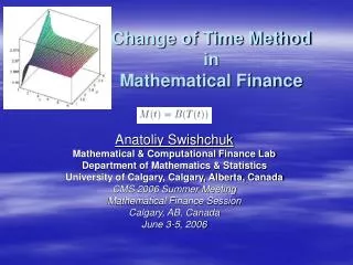
Change of Time Method in Mathematical Finance. Anatoliy Swishchuk Mathematical & Computational Finance Lab Department of Mathematics & Statistics University of Calgary, Calgary, Alberta, Canada CMS 2006 Summer Meeting Mathematical Finance Session Calgary, AB, Canada June 3-5, 2006.

E N D
Change of Time MethodinMathematical Finance Anatoliy Swishchuk Mathematical & Computational Finance Lab Department of Mathematics & Statistics University of Calgary, Calgary, Alberta, Canada CMS 2006 Summer Meeting Mathematical Finance Session Calgary, AB, Canada June 3-5, 2006
Outline • Change of Time (CT): Definition and Examples • Change of Time Method (CTM):Short History • Black-Scholes by CTM (i.e., CTM for GBM) • Explicit Option Pricing Formula (EOPF) for Mean-Reverting Model (MRM) by CTM • Black-Scholes Formula as a Particular Case of EOPF for MRM • Modeling and Pricing of Variance and Volatility Swaps by CTM
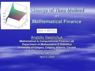
Change of Time: Definition and Examples • Change of Time-change time from t to a non-negative process with non-decreasing sample paths • Example 1 (Time-Changed Brownian Motion): M(t)=B(T(t)), B(t)-Brownian motion, T(t) is change of time • Example 2 (Subordinator): X(t) and T(t)>0 are some processes, then X(T(t)) is subordinated to X(t); T(t) is change of time • Example 3 (Standard Stochastic Volatility Model (SVM) ): M(t)=\int_0^t\sigma(s)dB(s), T(t)=[M(t)]=\int_0^t\sigma^2(s)ds.
Change of Time: Short History. I. • Bochner (1949) -introduced the notion of change of time (CT) (time-changed Brownian motion) • Bochner (1955) (‘Harmonic Analysis and the Theory of Probability’, UCLA Press, 176)-further development of CT
Change of Time: Short History. II. • Feller (1966) -introduced subordinated processes X(T(t)) with Markov process X(t) and T(t) as a process with independent increments (i.e., Poisson process); T(t) was called randomized operational time • Clark (1973)-first introduced Bochner’s (1949) time-changed Brownian motion into financial economics:he wrote down a model for the log-price M as M(t)=B(T(t)), where B(t) is Brownian motion, T(t) is time-change (B and T are independent)
Change of Time: Short History. III. • Ikeda & Watanabe (1981)-introduced and studied CTM for the solution of Stochastic Differential Equations • Carr, Geman, Madan & Yor (2003)-used subordinated processes to construct SV for Levy Processes (T(t)-business time)
Expression for C_T C_T=BS(T)+A(T) (Black-Scholes Part+Additional Term due to mean-reversion)
Dependence of ES(t) on S_0 and T(mean-reverting level L^*=2.569)
Brockhaus and Long Results • Brockhaus & Long (2000) obtained the same results for variance and volatility swaps for Heston model using another technique (analytical rather than probabilistic), including inverse Laplace transform
Statistics on Log Returns of S&P Canada Index (Jan 1997-Feb 2002)
Conclusions • CTM works for: • Geometric Brownian motion (to price options in money markets) • Mean-Reverting Model (to price options in energy markets) • Heston Model (to price variance and volatility swaps) • Much More: Covariance and Correlation Swaps
The End/Fin Thank You!/ Merci Beaucoup!