FORECAST SST TROP. PACIFIC (multi-models, dynamical and statistical)
270 likes | 450 Vues
IRI DYNAMICAL CLIMATE FORECAST SYSTEM. 2-tiered OCEAN ATMOSPHERE. GLOBAL ATMOSPHERIC MODELS ECPC(Scripps) ECHAM4.5(MPI) CCM3.x(NCAR) NCEP(MRF9) NSIPP(NASA) COLA2.x. PERSISTED GLOBAL SST ANOMALY. Persisted SST Ensembles 3 Mo. lead. 10. POST

FORECAST SST TROP. PACIFIC (multi-models, dynamical and statistical)
E N D
Presentation Transcript
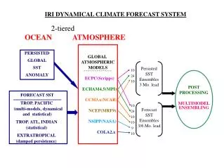
IRI DYNAMICAL CLIMATE FORECAST SYSTEM 2-tiered OCEAN ATMOSPHERE GLOBAL ATMOSPHERIC MODELS ECPC(Scripps) ECHAM4.5(MPI) CCM3.x(NCAR) NCEP(MRF9) NSIPP(NASA) COLA2.x PERSISTED GLOBAL SST ANOMALY Persisted SST Ensembles 3 Mo. lead 10 POST PROCESSING MULTIMODEL ENSEMBLING 24 10 FORECAST SST TROP. PACIFIC (multi-models, dynamical and statistical) TROP. ATL, INDIAN (statistical) EXTRATROPICAL (damped persistence) 10 Forecast SST Ensembles 3/6 Mo. lead 24 10 10 9 10
Empirical tools also used Mason & Goddard, 2001, Bull.Amer.Meteor.Soc.
Forecasts of the climate The tercile category system: Below, near, and above normal Probability: 33% 33% 33% Below| Near | Below| Near | Above Below| Near | | || ||| ||||.| || | | || | | | . | | | | | | | | | | Data: 0 10 20 30 40 50 60 70 80 90 100 110 120 130 140 150 160 170 180 190 200 Rainfall Amount (mm) (30 years of historical data for a particular location & season)
Monthly issued probability forecasts of seasonal global precipitation and temperature Four lead times - example: OCT | Nov-Dec-Jan* Dec-Jan-Feb Jan-Feb-Mar Feb-Mar-Apr *probabilities of extreme (low and high) 15% issued also
Sources of the Global Sea Surface Temperature Forecasts Tropical Pacific Tropical Atlantic Indian Ocean Extratropical Oceans NCEP Coupled CPTEC Statistical IRI Statistical Damped PersistenceLDEO Coupled Constr Analogue Atmospheric General Circulation Models Used in the IRI's Seasonal Forecasts, for Superensembles Name Where Model Was Developed Where Model Is Run NCEP MRF-9 NCEP, Washington, DC QDNR, Queensland, AustraliaECHAM 4.5 MPI, Hamburg, Germany IRI, Palisades, New YorkNSIPP NASA/GSFC, Greenbelt, MD NASA/GSFC, Greenbelt, MDCOLA COLA, Calverton, MD COLA, Calverton, MD ECPC SIO, La Jolla, CA SIO, La Jolla, CA CCM3.x NCAR, Boulder, CO NCAR, Boulder, CO (forthcoming) GFDL, Princeton, NJ GFDL or IRI
Ranked Probability Skill Score (RPSS) 3 RPSfcst = (Fcsticat – Obsicat)2 icat=1 icat ranges from 1 (below normal) to 3 (above normal) RPSS = 1 - (RPSfcst / RPSclim)
RPSS Skill of Individual Model Simulations: JAS 1950-97 Precipitation
Real-time Forecast Skill
Real-time Forecast Skill
Reliability Diagram longer “AMIP” period from Goddard et al. 2003 (EGS-AGU-EUG)
IRI uses two multi-model ensembling methods: Bayesian method Canonical variate method Both methods analyze historical model performance in responding to observed SST. Next: Bayesian weighting method for multi-model ensembling
Likelihood Rajagopalan et al., 2002:. Mon. Wea. Rev. k* represents the category that was observed at time t "a multi-year product of the probabilities that were hindcast for the category that was observed..." • Dirichlet distribution is appropriate for a multinomial process (i.e. terciles) • Combination of a and b is also Dirichlet with parameter a+b
Ways to compute weights Individual GCM + Climatology: 1 Effective sample sizes Multiple GCMs + Climatology: 2
Combine the individual weights from several models using a Two-Stage scheme: 3 (a) For each model in turn: (b) For the pooled ensemble thus created: Final weights:
Combination Forecasts of Jul-Sep Precipitation JAS 2003 One-Stage Two-Stage Two-Stage Cross-Validated Two-Stage, xv, Spatial Smoothing
Canonical variate method: A kind of discriminant analysis. Input: ensemble mean, ensemble spread, ensemble skewness Algorithm finds linear combinations of predictors leading to each catergorical (tercile) result. Differences among the sets of predictor weights are maximized.
Multi-model ensembling of dynamical predictions appears to be slightly superior to currently used statistical tools at NOAA/NCEP/CPC
Most important current needs in IRI forecast system: Improvement of SST prediction in 2-tiered system 1) Tropical Pacific: better model consolidation, with development of multiple evolving scenarios 2) Outside tropical Pacific:“Smarter” persistence scenario, or multivariate statistical model (e.g. CCA) Use of 1-tiered climate model for some regions Slab ocean model in locations where 2-tiered system fails (Indian Ocean, far west Pacific and tropical Atlantic oceans)