Download
1 / 52
520 likes | 613 Vues
Learn about advantages of fuzzy logic controllers, configuration components, choice of variables, and knowledge base design for efficient control systems. Discover how to set up the fuzzification and knowledge base components effectively for optimal performance.

E N D
10.1 Fuzzy logic controller • 10.1.1 Advantage of fuzzy logic controller • Useful cases (1)The control processes are too complex to analyze by conventional quantitative techniques. (2) The available sources of information are interpreted qualitatively, inexactly, or uncertainly. • Advantage of FLC (1) Parallel or distributed control • multiple fuzzy rules – complex nonlinear system (2) Linguistic control • linguistic terms - human knowledge (3) Robust control • more than 1 control rules – a error of a rule is not fatal
Knowledge base Input Fuzzification interface Defuzzification interface Output Inference State variable Controlled system (process) Control variable Control output Control input 10.1.2 Configuration of fuzzy logic controller • Fig 10.1 Configuration of FLC
10.1.2 Configuration of fuzzy logic controller • Four main components (1) The fuzzification interface : transforms input crisp values into fuzzy values (2)The knowledge base : contains a knowledge of the application domain and the control goals. (3) The decision-making logic :performs inference for fuzzy control actions (4) The defuzzification interface
10.1.3 Choice of state variables and control variables • State variables • input variables of the fuzzy control system • state, state error, state error deviation, and state error integral are often used • Control variables • output variables of the fuzzy control system • Selection of the variables • depends on expert knowledge on the process
10.2 Fuzzification interface component • Scale mapping of input data • convert the range of values of input variables into corresponding universe of discourse. • Strategy for noise • When observed data were disturbed by random noise, a fuzzification operator should convert the probabilistic data into fuzzy numbers. • a fuzzy singleton • assume that the observed data do not contain vagueness • a precise value and no fuzziness
10.2 Fuzzification interface component • Selection of fuzzification function x = fuzzifier (x0) • x0 is a observed crisp value • x is a fuzzy set • fuzzifier represents a fuzzification operator
F(x) 1 x x0 F(x) 1 x x0 base 10.2 Fuzzification interface component • fuzzification functions Fig 10.1 Fuzzification function for fuzzy singleton Fig 10.2 Fuzzification function for fuzzy triangular number
10.3 Knowledge base component • 10.3.1 Data base • Principal design parameters for an FLC • discretization and normalization of universe of discourse • fuzzy partition of input and output spaces • membership function of primary fuzzy set
10.3.1 Data base (1) Discretization of a universe of discourse • quantization • The quantization discretizes a universe into a certain number of segments. • Each segment is labeled as a generic element and forms a discrete universe. • A fuzzy set is then defined on the discrete universe of discourse. • The number of quantization levels affects an important influence on the control performance, • discretization • A scale mapping serves to transform measured variables into values in the discretized universe. • The mapping can be uniform (linear), non-uniform (nonlinear), or both.
Range Level No. x 2.4 6 2.4 x 2.0 5 1.6 x 0.8 4 0.8 x 0.4 3 0.4 x 0.2 2 0.2 x 0.1 1 0.1 x +0.1 0 0.1 x 0.2 1 0.2 x 0.4 2 0.4 x 0.8 3 0.8 x 1.1 4 1.1 x 1.4 5 1.4 x 6 Discretization and normalization of universe of discourse • Table 10.1 An example of discretization • a universe of discourse is discretized into 13 levels (-6, -5, -4, … , 0, 1, … , 5, 6).
Discretization and normalization of universe of discourse (2) Normalization of a universe of discourse • a discretization into a normalized universe. • The normalized universe consists of finite number of segments. • The scale mapping can be uniform, nonuniform, or both.
Range Normalized segments Normalized universe [6.9, 4.1] [1.0, 0.5] [4.1, 2.2] [0.5, 0.3] [2.2, 0.0] [0.3, 0.0] [1.0, 1.0] [0.0, 1.0] [0.0, 0.2] [1.0, 2.5] [0.2, 0.6] [2.5, 4.5] [0.6, 1.0] Discretization and normalization of universe of discourse • Table 10.2 shows an example • the universe of discourse [-6.9, +4.5] is transformed into the normalized closed interval [-1, 1].
10.3.1 Data base (3) Fuzzy partition of input and output spaces • linguistic variable • in the antecedent of a rule forms a fuzzy input space, • in the consequent of the rule forms a fuzzy output space. • In general, associated with a term set. • fuzzy partition of the space • determines how many terms should exist in a term set. • to find the number of primary fuzzy sets(linguistic terms)
NB NM NS ZE PS PM PB 1 0 1 Z N P 1 0 1 10.3.1 Data base • Fig 10.3 Example of fuzzy partition with linguistic terms 7 linguistic terms are often used • NB: negative big • NM: negative medium • NS: negative small • ZE: zero • PS: positive small • PM: positive medium • PB: positive big N: negative, Z: zero, P: positive NB, NM, NS, ZE, PS, PM, PB
x2 PS ZO NS NB x1 NB NS ZO PS PB x2 big small x1 small big 10.3.1 Data base • Fuzzy partition of input and output spaces Fig 10.4 A fuzzy partition in 2-dimension input space the maximum number of control rules = 20 (5x4) Fig 10.5 A fuzzy partition having three rules
Level No. NB NM NS ZE PS PM PB 6 1.0 0.3 0.0 0.0 0.0 0.0 0.0 5 0.7 0.7 0.0 0.0 0.0 0.0 0.0 4 0.3 1.0 0.3 0.0 0.0 0.0 0.0 3 0.0 0.7 0.7 0.0 0.0 0.0 0.0 2 0.0 0.3 1.0 0.3 0.0 0.0 0.0 1 0.0 0.0 0.7 0.7 0.0 0.0 0.0 0 0.0 0.0 0.3 1.0 0.3 0.0 0.0 1 0.0 0.0 0.0 0.7 0.7 0.0 0.0 2 0.0 0.0 0.0 0.3 1.0 0.3 0.0 3 0.0 0.0 0.0 0.0 0.7 0.7 0.0 4 0.0 0.0 0.0 0.0 0.3 1.0 0.3 5 0.0 0.0 0.0 0.0 0.0 0.7 0.7 6 0.0 0.0 0.0 0.0 0.0 0.3 1.0 10.3.1 Data base • Membership function of primary fuzzy set • Table 10.3 Definition of triangular membership function Term NM NM(6) = 0.3 NM(5) = 0.7 NM(4) = 1.0 NM(3) = 0.7 NM(2) = 0.3
Normalized universe Normalized segments mf f Fuzzy sets [1.0, 0.5] 1.0 0.4 NB [0.5, 0.3] 0.5 0.2 NM [0.3, 0.0] 0.2 0.2 NM [1.0, 1.0] [0.0, 0.2] 0.0 0.2 ZE [0.2, 0.6] 0.2 0.2 PS [0.6, 0.8] 0.5 0.2 PM [+0.8, +1.0] 1.0 0.4 PB 10.3.1 Data base • bell shaped membership function Table 10.4 Definition of bell-shaped membership function ; mean mf and standard deviation
NB NM NS ZE PS PM PB 1 0 1 10.3.1 Data base • Fig 10.6 Example of bell-shaped membership function
10.3.2 Rule base • Source of fuzzy control rules • derivation of fuzzy control rules • a heuristic method • rules are formed by analyzing the behavior of a controlled process. • The derivation relies on the qualitative knowledge of process behavior. • a deterministic method • can systematically determine the linguistic structure of rules.
10.3.2 Rule base • 4 modes of derivation of fuzzy control rules • Expert experience and control engineering knowledge: operating manual and questionnaire • Based on operators’ control actions : observation of human controller’s actions in terms of input-output operating data • Based on the fuzzy model of a process : linguistic description of the dynamic characteristics of a process • Based on learning : ability to modify control rules such as self-organizing controller
10.3.2 Rule base 2) Types of fuzzy control rules (1) State evaluation fuzzy control rules: • a collection of rules of the form(MISO version) R1: if x is A1, … and y is B1 then z is C1 R2: if x is A2, … and y is B2 then z is C2 … Rn: if x is An, … and y is Bn then z is Cn where x, … y and z are linguistic variables representing the process state variable and the control variable. Ai, … Bi and Ci are linguistic values of the variables x, … y and z in the universe of discourse U, … V and W, respectively i = 1, 2, … , n. That is, x U, Ai U, …, y V, Bi V, z W, Ci W
10.3.2 Rule base • general version, : the consequent part is represented as a function of the state variable x, …y. Ri: if x is Ai, … and y is Bi then z = fi(x, … y) • The state evaluation rules evaluate the process state (e.g. state, state error, change of error) at time t and compute a fuzzy control action at time t. • In the input variable space, the combination of input linguistic term may give a fuzzy rule. • a set of fuzzy rules Ri: if x is Ai, and y is Bi then z is Ci, i = 1, 2, … , n
y Bn C6 … Cn C5 C5 B2 C3 C4 C4 B1 C1 C2 … C7 A1 A2 … An x 10.3.2 Rule base • Fig 10.7 Fuzzy rules represented by a rule table
2) Types of fuzzy control rules(Con’t) (2) Object evaluation fuzzy control rules : predict present and future control actions, and evaluate control objectives (predictive fuzzy control) • Typical rules R1: if (z is C1 (x is A1 and y is B1)) then z is C1. … Rn: if (z is Cn (x is An and y is Bn)) then z is Cn. • A control action is determined by an objective evaluation that satisfies the desired states and objectives. • x and y are performance indices for the evaluation and z is control command. • Ai and Bi are fuzzy values such as NM and PS. • The most likely control rule is selected through predicting the results (x, y) corresponding to every control command Ci, i = 1, 2, … , n.
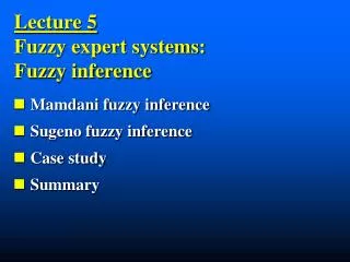
10.4 Inference (Decision making logic) • 10.4.1 Mandani method • minimum operator for a fuzzy implication • max-min operator for the composition Ri: if x is Ai and y is Bi then z is Ci, i = 1, 2, … , n x U, Ai U, y V, Bi V, z W, Ci W 1) When input data are singleton such as x = x0 and y = y0 the matching degree of rule Ri : the result of rule Ri : the aggregated result :
10.4 Inference (Decision making logic) 2) When input data are fuzzy sets, A and B the aggregated result :
10.4 Inference (Decision making logic) • 10.4.2 Larsen method • product operator(•) for a fuzzy implication • max-product operator for the composition 1) When input data are singleton such as x = x0 and y = y0 the matching degree of rule Ri : the result of rule Ri : the aggregated result :
10.4 Inference (Decision making logic) 2) When input data are fuzzy sets, A and B the matching degree of rule Ri : the result of rule Ri : the aggregated result :
10.4 Inference (Decision making logic) • 10.4.3 Tsukamoto method • the consequent part : fuzzy set with a monotonic membership function the result of rule Ri : the aggregated result :
1 =z2 5 7 1 3 7 9 z =(z1)2 5 7 10 1 3 7 9 z 8 10 3 z 5 8 10 5 z 7 10.4 Inference (Decision making logic) • Fig 10.8 Example of Tsukamoto control rules R1 : R2 : R3 : R4 :
10.4 Inference (Decision making logic) • 10.4.4 TSK method • the consequent part is given as a function of input variables. Ri: if x is Ai and y is Bi then z is fi(x, y) ,where z = f(x, y) is a crisp function of input variables x and y. When input data are singleton x0 and y0, then the inferred result of rule Ri is fi(x0, y0). the aggregated result : weighted average using the matching degree i
10.5 Defuzzification • Defuzzification • In many practical applications, a control command is given as a crisp value. • a process to get a non-fuzzy control action that best represents the possibility distribution of an inferred fuzzy control action. • no systematic procedure for choosing a good defuzzification strategy, • select one in considering the properties of application case
(z) z0 z 10.5.1 Mean of maximum method (MOM) • The MOM strategy generates a control action which represents the mean value of all control actions, whose membership functions reach the maximum. zj: control action whose membership functions reach the maximum. k: number of such control actions.
(z) z0 z 10.5.2 Center of area method (COA) • The widely used COA strategy generates the center of gravity of the possibility distribution of a fuzzy set C . n : the number of quantization levels of the output C : a fuzzy set defined on the output dimension (z)
10.5.3 Bisector of area (BOA) • The BOA generates the action (z0) which partitions the area into two regions with the same area . • = min{z | z W} = max{z | z W}
10.5.4 Lookup table • Lookup Table • Due to the problem of time complexity, it takes much time to compute the fuzzy inference and defuzzification. • simply shows relationships between input variables and control output actions. • can be constructed after making the FLC and identifying the relationships between the input and output variables. • In general, it is extremely difficult to get an acceptable lookup table of a nonlinear control system without constructing a corresponding FLC.
ce e 1.0 0.5 0 0.5 1.0 1.0 1.0 0.5 0.5 0.5 0.5 0.5 1.0 1.0 0.5 0.5 0.5 0 1.0 1.0 0.5 0.5 0.5 0.5 0.5 0.5 1.0 1.0 1.0 1.0 0.5 0.5 0.5 1.0 1.0 10.5.4 Lookup table • Example 10.1 the two input variables error (e) and change of error (ce), and control variable (v). when e = 1.0 and ce = 0.5, we can obtain v = 0.5
10.6 Design procedure of fuzzy logic controller 1) Determination of state variables and control variables 2) Determination of inference method 3) Determination of fuzzification method 4) Discretization and normalization of state variable space 5) Partition of variable space. 6) Determination of the shapes of fuzzy sets 7) Construction of fuzzy rule base 8) Determination of defuzzification strategy 9) Test and tuning 10) Construction of lookup table
10.7 Application example of FLC design • The control problem of Servomotors • Servomotors are used in many automatic system including drivers for printers, floppy disks, tape recorders, and robot manipulations. • The servomotor process shows nonlinear properties • We apply the fuzzy logic control to the motor control. • The task of the control is to rotate the shaft of the motor to a set point without overshoot.
10.7 Application example of FLC design • Design procedure for servomotor control 1) Determination of state variables and control variable (1) State variables (input variable of FLC): - Error : the set point minus the process output (e). - Change of error (ce) : the error from the process output minus the error from the last process output. (2) Control variable(output variable of FLC): - Control input (v) : the voltage applied to the process. 2) Determination of inference method • The Mandani inference method is selected 3) Determination of fuzzification method • fuzzy singleton : measure the state variables without uncertainty
10.7 Application example of FLC design 4)Discretization and normalization • The shaft encoder of the motor has a resolution of 1000. • The universes of discourse are as follows: 1000 e 1000 100 ce 100 • The servo amplifier has an output range of 30 V and thus the control variables (v) are in the range 30 v 30 • We discretize and normalize the input variables in the range [1, 1] as shown in Table 10.6(next page). • The control variable v is normalized in the range [1, 1] with the equation
error (e) error change (ce) quantized level 1000 e 800 100 ce 80 1.0 800 e 600 80 ce 60 0.8 600 e 400 60 ce 40 0.6 400 e 200 40 ce 20 0.4 200 e 100 20 ce 10 0.2 100 e 100 10 ce 10 0 100 e 200 10 ce 20 0.2 200 e 400 20 ce 40 0.4 400 e 600 40 ce 60 0.6 600 e 800 60 ce 80 0.8 800 e 1000 80 ce 100 1.0 10.7 Application example of FLC design 4)Discretization and normalization(con’t) Table 10.6 Discretization and normalization
NB NM NS ZE PS PM PB 1 0 1 e ce v 10.7 Application example of FLC design 5) Partition of input space and output space • We partition space of each input and output variable into seven regions, • Each region is associated with linguistic term as shown in Fig 10.13. • the maximum number of possible fuzzy rules is 49. Fig 10.13 Partition of space
Level NB NM NS ZE PS PM PB 1 1 0.5 0 0 0 0 0 0.8 0 1 0 0 0 0 0 0.6 0 0.5 0.5 0 0 0 0 0.4 0 0 1 0 0 0 0 0.2 0 0 0.5 0.5 0 0 0 0 0 0 0 1 0 0 0 0.2 0 0 0 0.5 0.5 0 0 0.4 0 0 0 0 1 0 0 0.6 0 0 0 0 0.5 0.5 0 0.8 0 0 0 0 0 1 0 1.0 0 0 0 0 0 0.5 1 10.7 Application example of FLC design 6) Determination of the shapes of fuzzy sets • We normalized the input and output variables on the same interval [-1, +1] and partitioned the region into seven subregions Table 10.7 Definition of primary fuzzy sets
NB NM NS ZE PS PM PB 1 0.5 1 0.8 0.6 0.4 0.2 0 0.2 0.4 0.6 0.8 1.0 10.7 Application example of FLC design • Fig 10.14 Graphical representation of primary fuzzy sets
10.7 Application example of FLC design 7) Construction of fuzzy rules • We interviewed with an expert of the servomotor control, and we collect knowledge such as: “If the error is zero and the error change is positive small, then the control input is negative small” (1)If e is PB and ce is any, then v is PB. (2)If e is PM and ce is NB, NM, or NS, then v is PS. (3)If e is ZE and ce is ZE, PS, or PM, then v is ZE. (4)If e is PS and ce is NS, ZE, or PS, then v is ZE. (5)If e is NS and ce is NS, ZE, PS, or PM, then v is NS. (6) If e is NS or ZE and ce is PB, then v is PS.
ce NB NM NS ZE PS PM PB e NB NB NM NM NS NS PS ZE NS ZE PS PM PM PS PB PB 10.7 Application example of FLC design • Construction of fuzzy rules(Con’t) Fig 10.15 Fuzzy rule table
10.7 Application example of FLC design 8) Determination of defuzzification strategy • We take the COA (center of area) method because it is most commonly used. 9) Test and tuning • We checked the performance of the developed controller and refined some fuzzy rules. 10) Construction of lookup table • For example, for c = -0.2 and ce = 0, v is -0.4 for c = -0.4 and ce = 0.4, v is 0.2 • this lookup table can be used in order to save the inference time and defuzzification time
Knowledge base User input Fuzzification interface Linguistic approximation Output Scheduler Inference engine 10.8 Fuzzy expert systems • Configuration of fuzzy expert system