Download
1 / 14
140 likes | 327 Vues
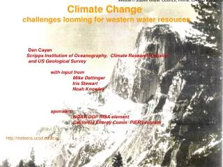
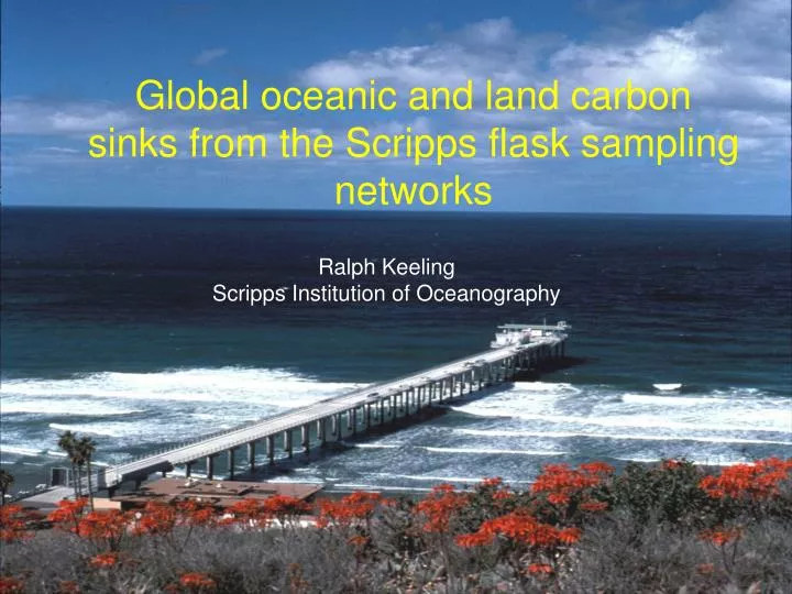
Global oceanic and land carbon sinks from the Scripps flask sampling networks. Ralph Keeling Scripps Institution of Oceanography. F. B. O. Fossil-fuel burning. Land photosynthesis & respiration. Ocean CO 2 uptake: H 2 O + CO 2 + CO 3 = ↔ 2HCO 3 -. Atmospheric CO 2 budget.

E N D
Global oceanic and land carbon sinks from the Scripps flask sampling networks Ralph KeelingScripps Institution of Oceanography
F B O Fossil-fuel burning Land photosynthesis & respiration Ocean CO2 uptake: H2O + CO2 + CO3= ↔ 2HCO3- Atmospheric CO2 budget ΔCO2 = F – O – B
F B O Fossil-fuel burning: CHy + (1+y/4)O2 → CO2 + (y/2)H2O Land photosynthesis & respiration: CO2 + H2O ↔ O2 + H2O Ocean CO2 uptake: H2O + CO2 + CO3= ↔ 2HCO3- Atmospheric CO2 and O2 budgets ΔCO2 = F – O – B ΔO2 = -1.4F + 1.1B
F B O Fossil-fuel burning: CHy + (1+y/4)O2 → CO2 + (y/2)H2O Land photosynthesis & respiration: CO2 + H2O ↔ O2 + H2O Ocean CO2 uptake: H2O + CO2 + CO3= ↔ 2HCO3- Atmospheric CO2 and O2 budgets ΔCO2 = F – O – B ΔO2 = -1.4F + 1.1B + Z Z
Recent O2 based Carbon budgets Time Outgas Ocean Land Period Corr. Sink Sink Manning (2001) 1990-2000 0.10 1.68±0.5 1.44±0.7 & IPCC(2001) Keeling & 1990-2000 0.28 1.86 ± 0.6 1.26±0.8 Garcia (2002) Manning & 1993-2003 0.48 2.24 ± 0.61 0.51±0.74 Keeling (2005, submitted) Units: Pg C yr-1
Recent O2 based Carbon budgets Time Outgas Ocean Land Period Corr. Sink Sink Manning (2001) 1990-2000 0.10 1.68±0.5 1.44±0.7 & IPCC(2001) Keeling & 1990-2000 0.28 1.86 ± 0.6 1.26±0.8 Garcia (2002) Manning & 1993-2003 0.48 2.24 ± 0.61 0.51±0.74 Keeling (2005, submitted) Units: Pg C yr-1 Increase in estimated ocean sink results from (1) Upwards revision of outgassing correction, as indicated. (2) Observed O2 loss rate higher over 2000-2003 period.
Interannual variations in CO2 O2/N2 and 13C/12C Correlations between CO2, δ13C, and O2 imply land dominance of variability on El Nino time scales
Discussion: Dominance of land to interannual variability also supported by atmospheric inversions. This is now beyond dispute. Nevertheless, the smaller oceanic contribution to variability remains poorly resolved. All available approaches have problems: CO2 Inversions: can’t distinguish well between coastal oceans and land fluxes. 13C/12C: complicated by possible variations in isotopic fractionation factor with land biota changes. O2: complicated by interannual variations in air-sea O2 exchange.
ΔCO2 = F – O – B ΔO2 = -1.4F + 1.1B + Z ΔO2 +1.1ΔCO2 = -0.3F -1.1O + Z Discussion, continued: Measurements of O2 nevertheless may prove helpful, by providing a test of ocean models that predict CO2 variability. The test is realizable via the tracer APO = O2 + 1.1 CO2 Z = Air-sea O2 flux Interannual variability in APO should reflect interannual variability in the combined air-sea CO2 and O2 flux, since interannual variability in fossil-fuel burning (F) is small.
Observed versus Modeled variations in APO Summary of findings: Relatively good model-to-model agreement. Observations show ~ ~2x more variability. If models underestimate APO variability, do they also underestimate CO2 variability? Needs more work to resolve.
Acknowledgements Charles D KeelingAndrew ManningRoberta HammeBill PaplawskyGalen McKinley Mick Follows Corinne LeQuere Christian Roedenbeck Laurent Bopp
Ocean biogeochem. Models MPI Jena model Authors: Buitenhuis, LeQuere, Rodgers Physics: OPA-ORCA Bio model: Dynamic Green Ocean type Forcing: daily NCEP Resolution: 0.5°x2° tropics and poles 2°x2° sub-tropics Gas exchange: Liss and Merlivat IPSL model Authors: Bopp, Rodgers Physics: OPA-ORCA Bio model: Dynamic Green Ocean type Forcing: daily NCEP, mixed boundary conditions Resolution:0.5°x2° tropics and poles 2°x2° sub-tropics Gas exchange: Wanninkhov (1992) MIT model Authors: McKinley, Follows, Marshall Physics: MITgcm-ECCO Biogeo: phosphate & light based export Forcing: 12 hr NCEP Resolution: 1°x1° extra-tropics 0.3°x1° tropics Gas exchange: Wanninkhov (1992)