Introduction to Large Sparse Graphs: Structure, Applications, and Power Laws
This document explores the fundamentals of large sparse graphs, focusing on their structure and applications within various domains, including urban networks, social interactions, and biological systems. It emphasizes the significance of graph models, particularly in understanding complex relationships, such as flights between cities and connections between individuals based on various factors. The analysis delves into characteristics like small-world phenomena, power-law degree distributions, and the historical context of graph theory. This comprehensive overview aids in grasping the complexities of massive, dynamic graphs.

Introduction to Large Sparse Graphs: Structure, Applications, and Power Laws
E N D
Presentation Transcript
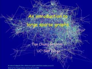
An introduction to large sparse graphs Fan Chung Graham UC San Diego
edge vertex A graph G = (V,E)
Vertices cities Edges flights Graph models _____________________________
Vertices cities people Edges flights pairs of friends Graph models _____________________________
Vertices cities people telephones Edges flights pairs of friends phone calls Graph models _____________________________
Vertices cities people telephones web pages genes Edges flights pairs of friends phone calls linkings regulatory effects Graph models _____________________________
Graph Theory has 250 years of history. Leonhard Euler, 1707-1783
Geometric graphs Algebraic graphs
Geometric graphs Algebraic graphs General graphs By Bill Cheswick
Geometric graphs Algebraic graphs Real graphs (router graph)
Geometric graphs Algebraic graphs Real graphs (protein interactions by Jawoong Jeong)
Geometric graphs Algebraic graphs Real graphs (Web Cashe map by Bradley Huffaker)
Geometric graphs Algebraic graphs Real graphs Collaboration graph
Massive data Massive graphs
Massive data Massive graphs The information we deal with is taking on a networked character.
Massive data Massive graphs • WWW-graphs • a. Bill Cheswick
Massive data Massive graphs • WWW-graphs • Call graphs • Acquaintance graphs a. Part of the collaboration graph
Massive data Massive graphs • WWW-graphs • Call graphs • Acquaintance graphs • Graphs from any data a.base
What does a massive graph look like? sparse clustered small diameter
What does a massive graph look like? sparse clustered small diameter prohibitively large dynamically changing incomplete information
What does a massive graph look like? sparse clustered small diameter prohibitively large dynamically changing incomplete information Hard to describe ! Harder to analyze !!
Some prevailing characteristic of large realistic networks • Small world phenomenon Small diameter/average distance Clustering • Power law degree distribution
A crucial observation Discovered by several groups independently. • Barabási, Albert and Jeung, 1999. • Broder, Kleinberg, Kumar, Raghavan, Rajagopalan aaand Tomkins, 1999. • M Faloutsos, P. Faloutsos and C. Faloutsos, 1999. • Abello, Buchsbaum, Reeds and Westbrook, 1999. • Aiello, Chung and Lu, 1999. Massive graphs satisfy the power law.
Massive graphs satisfy the power law. Power decay degree distribution. The degree sequences satisfy thepower law: The number of vertices of degree j is proportional to j- where is some constant 2.
A random graph model for a power law graphs Two parameters: and P(,) : a random power law graph. : log size : log log growth rate
A random graph model for a power law graphs Two parameters: and P(,) : a random power law graph. P(,) assigns uniform probability to all graphs satisfying: log y - log x where y = the number of vertices with degree x.
Comparisons From real data From simulation
The history of power law • Zipf’s law, 1949. (The nth most frequent word occurs at rate 1/n) • Yule’s law, 1942. • Lotka’s law, 1926. (distribution of authors in chemical abstracts) • Pareto, 1897 (Wealth distribution follows a power law.) (City population follows a power law.) 1907-1916 Natural language Bibliometrics Social sciences Nature
Examples of power law • Inter • Internet graphs. • Call graphs. • Collaboration graphs. • Acquaintance graphs. • Language usage
The collaboration graph is a power law graph, based on data from Math Review with 337451 authors with power 2.55
Collaboration graph (Math Review) • 337,000 authors • 496,000 edges • Average 5.65 collaborations per person • Average 2.94 collaborators per person • Maximum degree 1401 • A giant component of size 208,000 • 84,000 isolated vertices
Collaboration graph (Math Review) • 337,000 authors • 496,000 edges • Average 5.65 collaborations per person • Average 2.94 collaborators per person • Maximum degree 1401. • A giant component of size 208,000 • 84,000 isolated vertices Guess who?
An induced subgraph of the collaboration graph with authors of Erdös number ≤ 2.
Occurrences of words in WSJ Collection, a 131.6 MB collection of 46449 newspaper articles aaaa (19 million terms). Top 50 terms are included here.