Download
1 / 82
1.02k likes | 1.67k Vues
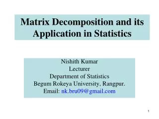
Matrix Decomposition and its Application in Statistics. Nishith Kumar Lecturer Department of Statistics Begum Rokeya University, Rangpur. Email: nk.bru09@gmail.com. Overview. Introduction LU decomposition QR decomposition Cholesky decomposition Jordan Decomposition

E N D
Matrix Decomposition and its Application in Statistics Nishith Kumar Lecturer Department of Statistics Begum Rokeya University, Rangpur. Email: nk.bru09@gmail.com
Overview • Introduction • LU decomposition • QR decomposition • Cholesky decomposition • Jordan Decomposition • Spectral decomposition • Singular value decomposition • Applications
Introduction Some of most frequently used decompositions are the LU, QR, Cholesky, Jordan, Spectral decomposition and Singular value decompositions. • This Lecture covers relevant matrix decompositions, basic numerical methods, its computation and some of its applications. • Decompositions provide a numerically stable way to solve a system of linear equations, as shown already in [Wampler, 1970], and to invert a matrix. Additionally, they provide an important tool for analyzing the numerical stability of a system.
Easy to solve system (Cont.) Some linear system that can be easily solved The solution:
Easy to solve system (Cont.) Lower triangular matrix: Solution: This system is solved using forward substitution
Easy to solve system (Cont.) Upper Triangular Matrix: Solution:This system is solved using Backward substitution
LU Decomposition LU decomposition was originally derived as a decomposition of quadratic and bilinear forms. Lagrange, in the very first paper in his collected works( 1759) derives the algorithm we call Gaussian elimination. Later Turing introduced the LU decomposition of a matrix in 1948 that is used to solve the system of linear equation. Let A be a m × m with nonsingular square matrix. Then there exists two matrices L and U such that, where L is a lower triangular matrix and U is an upper triangular matrix. and Where, J-L Lagrange (1736 –1813) A. M. Turing (1912-1954)
How to decompose A=LU? A…U (upper triangular) U = Ek E1 A A = (E1)-1 (Ek)-1U If each such elementary matrix Ei is a lower triangular matrices,it can be proved that (E1)-1,, (Ek)-1 are lower triangular, and(E1)-1 (Ek)-1is a lower triangular matrix.Let L=(E1)-1 (Ek)-1 then A=LU. U E2 E1 A
Calculation of L and U (cont.) Now reducing the first column we have =
Calculation of L and U (cont.) If A is a Non singular matrix then for each L (lower triangular matrix) the upper triangular matrix is unique but an LU decomposition is not unique. There can be more than one such LU decomposition for a matrix. Such as Now Therefore, = =LU =LU =
Calculation of L and U (cont.) Calculation of L and U (cont.) Thus LU decomposition is not unique. Since we compute LU decomposition by elementary transformation so if we change L then U will be changed such that A=LU To find out the unique LU decomposition, it is necessary to put some restriction on L and U matrices. For example, we can require the lower triangular matrix L to be a unit one (i.e. set all the entries of its main diagonal to ones). LU Decomposition in R: • library(Matrix) • x<-matrix(c(3,2,1, 9,3,4,4,2,5 ),ncol=3,nrow=3) • expand(lu(x))
Calculation of L and U (cont.) • Note: there are also generalizations of LU to non-square and singular matrices, such as rank revealing LU factorization. • [Pan, C.T. (2000). On the existence and computation of rank revealing LU factorizations. Linear Algebra and its Applications, 316: 199-222. • Miranian, L. and Gu, M. (2003). Strong rank revealing LU factorizations. Linear Algebra and its Applications, 367: 1-16.] • Uses: The LU decomposition is most commonly used in the solution of systems of simultaneous linear equations. We can also find determinant easily by using LU decomposition (Product of the diagonal element of upper and lower triangular matrix).
Solving system of linear equation using LU decomposition Suppose we would like to solve a m×m system AX = b. Then we can find a LU-decomposition for A, then to solve AX =b, it is enough to solve the systems Thus the system LY = b can be solved by the method of forward substitution and the system UX = Y can be solved by the method of backward substitution. To illustrate, we give some examples Consider the given system AX = b, where and
Solving system of linear equation using LU decomposition We have seen A = LU, where Thus, to solve AX = b, we first solve LY = b by forward substitution Then
Solving system of linear equation using LU decomposition Now, we solve UX =Y by backward substitution then
QR Decomposition If A is a m×n matrix with linearly independent columns, then A can be decomposed as , where Q is a m×n matrix whose columns form an orthonormal basis for the column space of A and R is an nonsingular upper triangular matrix. Firstly QR decomposition originated with Gram(1883). Later Erhard Schmidt (1907) proved the QR Decomposition Theorem Jørgen Pedersen Gram (1850 –1916) Erhard Schmidt (1876-1959)
QR-Decomposition (Cont.) Theorem : If A is a m×n matrix with linearly independent columns, then A can be decomposed as , where Q is a m×n matrix whose columns form an orthonormal basis for the column space of A and R is an nonsingular upper triangular matrix. Proof: Suppose A=[u1 | u2| . . . | un] and rank (A) = n. Apply the Gram-Schmidt process to {u1, u2 , . . . ,un} and the orthogonal vectors v1, v2 , . . . ,vn are Let for i=1,2,. . ., n. Thus q1, q2 , . . . ,qn form a orthonormal basis for the column space of A.
QR-Decomposition (Cont.) Now, i.e., Thus uiisorthogonal to qj for j>i;
QR-Decomposition (Cont.) Let Q= [q1 q2 . . . qn] , so Q is a m×n matrix whose columns form an orthonormal basis for the column space of A . Now, i.e., A=QR. Where, Thus A can be decomposed as A=QR , where R is an upper triangular and nonsingular matrix.
QR Decomposition Example: Find the QR decomposition of
Calculation of QR Decomposition Applying Gram-Schmidt process of computing QR decomposition 1st Step: 2nd Step: 3rd Step:
Calculation of QR Decomposition 4th Step: 5th Step: 6th Step:
Calculation of QR Decomposition Therefore, A=QR R code for QR Decomposition: x<-matrix(c(1,2,3, 2,5,4, 3,4,9),ncol=3,nrow=3) qrstr <- qr(x) Q<-qr.Q(qrstr) R<-qr.R(qrstr) Uses: QR decomposition is widely used in computer codes to find the eigenvalues of a matrix, to solve linear systems, and to find least squares approximations.
Least square solution using QR Decomposition The least square solution of b is Let X=QR. Then Therefore,
Cholesky Decomposition Cholesky died from wounds received on the battle field on 31 August 1918 at 5 o'clock in the morning in the North of France. After his death one of his fellow officers, Commandant Benoit, published Cholesky's method of computing solutions to the normal equations for some least squares data fitting problems published in the Bulletin géodesique in 1924. Which is known as Cholesky Decomposition Cholesky Decomposition: If A is a real, symmetric and positive definite matrix then there exists a unique lower triangular matrix L with positive diagonal element such that . Andre-Louis Cholesky 1875-1918
Cholesky Decomposition Theorem: If A is a n×n real, symmetric and positive definite matrix then there exists a unique lower triangular matrix G with positive diagonal element such that . Proof: Since A is a n×n real and positive definite so it has a LU decomposition, A=LU. Also let the lower triangular matrix L to be a unit one (i.e. set all the entries of its main diagonal to ones). So in that case LU decomposition is unique. Let us suppose observe that . is a unit upper triangular matrix. Thus, A=LDMT .Since A is Symmetric so, A=AT . i.e., LDMT =MDLT. From the uniqueness we have L=M. So, A=LDLT . Since A is positive definite so all diagonal elements of D are positive. Let then we can write A=GGT.
Cholesky Decomposition (Cont.) Procedure To find out the cholesky decomposition Suppose We need to solve the equation
Example of Cholesky Decomposition For k from 1 to n For j from k+1 to n Suppose Then Cholesky Decomposition Now,
R code for Cholesky Decomposition • x<-matrix(c(4,2,-2, 2,10,2, -2,2,5),ncol=3,nrow=3) • cl<-chol(x) • If we Decompose A as LDLT then and
Application of Cholesky Decomposition Cholesky Decomposition is used to solve the system of linear equation Ax=b, where A is real symmetric and positive definite. In regression analysis it could be used to estimate the parameter if XTX is positive definite. In Kernel principal component analysis, Cholesky decomposition is also used (Weiya Shi; Yue-Fei Guo; 2010)
Characteristic Roots and Characteristics Vectors Any nonzero vector x is said to be a characteristic vector of a matrix A, If there exist a number λ such that Ax= λx; Where A is a square matrix, also then λ is said to be a characteristic root of the matrix A corresponding to the characteristic vector x. Characteristic root is unique but characteristic vector is not unique. We calculate characteristics root λfrom thecharacteristic equation |A- λI|=0 For λ=λithe characteristics vectoris thesolution of x from the following homogeneous system of linear equation(A- λiI)x=0 Theorem: If A is a real symmetric matrix and λi and λj are two distinct latent root of A then the corresponding latent vector xi and xj are orthogonal.
Multiplicity Algebraic Multiplicity: The number of repetitions of a certain eigenvalue. If, for a certain matrix, λ={3,3,4}, then the algebraic multiplicity of 3 would be 2 (as it appears twice) and the algebraic multiplicity of 4 would be 1 (as it appears once). This type of multiplicity is normally represented by the Greek letter α, where α(λi) represents the algebraic multiplicity of λi. Geometric Multiplicity: the geometric multiplicity of an eigenvalue is the number of linearly independent eigenvectors associated with it.
Jordan DecompositionCamille Jordan (1870) • Let A be any n×n matrix then there exists a nonsingular matrix P and JK(λ) a k×k matrix form Such that Camille Jordan (1838-1921) where k1+k2+ … + kr =n. Also λi , i=1,2,. . ., r are the characteristic roots And kiare the algebraic multiplicity of λi , Jordan Decomposition is used in Differential equation and time series analysis.
Spectral Decomposition Let A be a m × m real symmetric matrix. Then there exists an orthogonal matrix P such that or , where Λ is a diagonal matrix. A. L. Cauchy established the Spectral Decomposition in 1829. CAUCHY, A.L.(1789-1857)
Spectral Decomposition and Principal component Analysis (Cont.) By using spectral decomposition we can write In multivariate analysis our data is a matrix. Suppose our data is X matrix. Suppose X is mean centered i.e., and the variance covariance matrix is ∑. The variance covariance matrix ∑ is real and symmetric. Using spectral decomposition we can write ∑=PΛPT . Where Λ is a diagonal matrix. Also tr(∑) = Total variation of Data =tr(Λ)
Spectral Decomposition and Principal component Analysis (Cont.) The Principal component transformation is the transformation Y=(X-µ)P Where, • E(Yi)=0 • V(Yi)=λi • Cov(Yi ,Yj)=0 if i ≠ j • V(Y1) ≥ V(Y2) ≥ . . . ≥ V(Yn)
R code for Spectral Decomposition x<-matrix(c(1,2,3, 2,5,4, 3,4,9),ncol=3,nrow=3) eigen(x) Application: • For Data Reduction. • Image Processing and Compression. • K-Selection for K-means clustering • Multivariate Outliers Detection • Noise Filtering • Trend detection in the observations.
Historical background of SVD There are five mathematicians who were responsible for establishing the existence of the singular value decomposition and developing its theory. Camille Jordan (1838-1921) James Joseph Sylvester (1814-1897) Erhard Schmidt (1876-1959) Hermann Weyl (1885-1955) Eugenio Beltrami (1835-1899) The Singular Value Decomposition was originally developed by two mathematician in the mid to late 1800’s 1. Eugenio Beltrami , 2.Camille Jordan Several other mathematicians took part in the final developments of the SVD including James Joseph Sylvester, Erhard Schmidt and Hermann Weyl who studied the SVD into the mid-1900’s. C.Eckart and G. Young prove low rank approximation of SVD (1936). C.Eckart
What is SVD? Any real (m×n) matrix X, where (n≤ m), can be decomposed, X = UΛVT • U is a (m×n) column orthonormal matrix (UTU=I), containing the eigenvectors of the symmetric matrix XXT. • Λ is a (n×n ) diagonal matrix, containing the singular values of matrix X. The number of non zero diagonal elements of Λ corresponds to the rank ofX. • VTis a (n×n) row orthonormal matrix (VTV=I), containing the eigenvectors of the symmetric matrix XTX.
Singular Value Decomposition (Cont.) Theorem (Singular Value Decomposition) : Let X be m×n of rank r, r ≤ n ≤ m. Then there exist matrices U , V and a diagonal matrix Λ, with positive diagonal elements such that, Proof: Since X is m × n of rank r, r ≤ n ≤ m. So XXT and XTX both ofrank r ( by using the concept of Grammian matrix ) and of dimension m × m and n × n respectively. Since XXT is real symmetric matrix so we can write by spectral decomposition, Where Q and D are respectively, the matrices of characteristic vectors and corresponding characteristic roots of XXT. Again since XTX is real symmetric matrix so we can write by spectral decomposition,
Singular Value Decomposition (Cont.) Where R is the (orthogonal) matrix of characteristic vectors and M is diagonal matrix of the corresponding characteristic roots. Since XXT and XTX are both of rank r, only r of their characteristic roots are positive, the remaining being zero. Hence we can write, Also we can write,
Singular Value Decomposition (Cont.) We know that the nonzero characteristic roots of XXT and XTX are equal so Partition Q, R conformably with D and M, respectively i.e., ; such that Qris m × r , Rris n × r and correspond respectively to the nonzero characteristic roots of XXT and XTX. Now take Where are the positive characteristic roots of XXT and hence those of XTX as well (by using the concept of grammian matrix.)
Singular Value Decomposition (Cont.) Now define, Now we shall show that S=X thus completing the proof. Similarly, From the first relation above we conclude that for an arbitrary orthogonal matrix, say P1 , While from the second we conclude that for an arbitrary orthogonal matrix, say P2 We must have
Singular Value Decomposition (Cont.) The preceding, however, implies that for arbitrary orthogonal matrices P1 , P2 the matrix X satisfies Which in turn implies that, Thus
R Code for Singular Value Decomposition x<-matrix(c(1,2,3, 2,5,4, 3,4,9),ncol=3,nrow=3) sv<-svd(x) D<-sv$d U<-sv$u V<-sv$v
Decomposition in Diagram Matrix A Full column rank Lu decomposition Not always unique QR Decomposition Rectangular Square Asymmetric Symmetric SVD AM=GM AM>GM PD Similar Diagonalization P-1AP=Λ Jordan Decomposition Cholesky Decomposition Spectral Decomposition
Properties Of SVD Rewriting the SVD where r = rank of A λi = the i-th diagonal element of Λ. ui and vi are the i-th columns of U and V respectively.
Proprieties of SVDLow rank Approximation Theorem: If A=UΛVT is the SVD of A and the singular values are sorted as , then for any l <r, the best rank-l approximation to A is ; Low rank approximation technique is very much important for data compression.
Low-rank Approximation • SVD can be used to compute optimal low-rank approximations. • Approximation of A is à of rank k such that If are the characteristics roots of ATA then à and X are both mn matrices. Frobenius norm
column notation: sum of rank 1 matrices Low-rank Approximation • Solution via SVD set smallest r-k singular values to zero K=2