Download
1 / 13
130 likes | 330 Vues
Incorporating Iterative Refinement with Sparse Cholesky. April 2007 Doron Pearl. Robustness of Cholesky. Recall the Cholesky algorithm – a lot of subtractions/additions cancellation and round-off errors accumulate

E N D
Incorporating Iterative Refinementwith Sparse Cholesky April 2007Doron Pearl
Robustness of Cholesky • Recall the Cholesky algorithm – a lot of subtractions/additions cancellation and round-off errors accumulate • Sparse Cholesky with Symbolic Factorization provides high performance – but what about accuracy and robustness?
Test case: IPM • All IPMs implementations involve solving a system of linear equations (ADATx=b) in each step. • Usually in IPM when approaching the optimum the ADAT matrix becomes ill-conditioned.
Direct A = LU Iterative y’ = Ay More General Non- symmetric Symmetric positive definite More Robust More Robust Less Storage Sparse Ax=b solvers
Iterative Refinement • A technique for improving a computed solution to a linear system Ax = b. • r is constructed in higher precision. • x2 should be more accurate (why?) Algorithm 0. (Solve Ax1=b someway – LU/Chol) Compute the residual r = b – Ax1 Solve the correction d in Ad = r Update the solution x2 = x1 + d
Iterative Refinement 1. L LT = chol(A) % Choleskey factorization (SINGLE) O(n3) 2. x = L\(LT\b) % Back solve (SINGLE) O(n2) 2. r = b – Ax % Residual (DOUBLE) O(n2) 3. while ( || r || not small enough ) %stopping criteria 3.1 d = L\(LT\r) % Choleskey fct. on the residual (SINGLE) O(n2) 3.2 x = x + d % new solution (DOUBLE) O(n2) 3.3 r = b - Ax % new residual (DOUBLE) O(n2) COST: (SINGLE) O(n3) + #ITER * (DOUBLE) O(n2) My implementation is available here: http://optlab.mcmaster.ca/~pearld/IterRef.cpp
Convergence rate of IR n=40, Cond. #: 3.2*106 0.00539512 0.00539584 0.00000103 0.00000000 n=60, Cond. #: 1.6*107 0.07641456 0.07512849 0.00126436 0.00002155 0.00000038 n=80 Cond#: 5*107 0.12418532 0.12296046 0.00121245 0.00001365 0.00000022 n=100, Cond#: 1.4*108 0.70543142 0.80596178 0.11470973 0.01616639 0.00227991 0.00032101 0.00004520 0.00000631 0.00000080
Convergence rate of IR N=250, Condition number: 1.9*109 4.58375704 1.664398 1.14157504 0.69412263 0.42573218 0.26168779 0.16020511 0.09874206 0.06026184 0.03725948 0.02276088 0.01405095 0.00857605 0.00526488 0.00324273 0.00198612 0.00121911 0.00074712 0.00045864 0.00028287… 0.00000172 ||Err||2 iteration For N>350, Cond#= 1.6*1011:No convergence
More Accurate With extra precise iterative refinement Conventional Gaussian Elimination 1/e e
Conjugate Gradient in a nutshell • Iterative method for solving Ax=b • Minimizes the a quadratic function:f(x) = 1/2xTAx-bTx+c • Choose search direction that are conjugated to each other. • In non-finite precision converges after n iterations. • But to solve efficiently CG needs a good preconditioners – not available for the general case.
Conjugate Gradient x0 = 0, r0 = b, p0 = r0 for k = 1, 2, 3, . . . αk = (rTk-1rk-1) / (pTk-1Apk-1) step length xk = xk-1 + αk pk-1 approx solution rk = rk-1 – αk Apk-1 residual βk = (rTk rk) / (rTk-1rk-1) improvement pk = rk + βk pk-1 search direction • One matrix-vector multiplication per iteration • Two vector dot products per iteration • Four n-vectors of working storage
Reference • John R. Gilbert, University of California. Talk at "Sparse Matrix Days in MIT“ • Exploiting the Performance of 32 bit Floating Point Arithmetic in Obtaining 64 bit Accuracy (2006); Julie Langou et. al, Innovative Computation Laboratory, Computer Science Department, University of Tennessee • “The Future of LAPACK and ScaLAPACK”Jim Demmel, UC Berkeley.