Mastering Games: Minimax Algorithm Insights
640 likes | 779 Vues
Explore game theory basics, AI applications in deterministic games, and Minimax search principles. Understand the complexities of search problems, decision-making strategies, and optimal gameplay in adversarial environments.

Mastering Games: Minimax Algorithm Insights
E N D
Presentation Transcript
Adversarial Search Berlin Chen 2004 References: 1. S. Russell and P. Norvig. Artificial Intelligence: A Modern Approach. Chapter 6 2. S. Russell’s teaching materials
Introduction • Game theory • First developed by von Neumann and Morgensten • Widely studied by economists, mathematicians, financiers, etc. • The action of one player (agent) can significantly affect the utilities of the others • Cooperative or competitive • Deal with the environments with multiple agents • Most games studied in AI are • Deterministic (but strategic) • Turn-taking • Two-player • Zero-sum • Perfect information (state, action(state)) → next state This means in deterministic, fully observable environments in which there are two agentswhose actions must alternate and in which the utility values at the end of game are always equal or opposite But not physical games
Types of Games Deterministic chance • Games are one of the first tasks undertaken in AI • The abstract nature of (nonphysical) games makes them an appealing subject in AI • Computers have surpassed humans on checkers and Othello, and have defeated human champions in chess and backgammon • However, in Go, computers still perform at the amateur level Perfect information Imperfect information
Games as Search Problems • Games are usually too hard to solve • E.g., a chess game • Average branching factor: 35 • Average moves by each player: 50 • Total number of nodes in the search tree: 35100 or 10154 • Total number of distinct states:1040 • The solution is a strategy that specifies a move for every possible opponent reply • Time limit: how to make the best possible use of time? • Calculating the optimal decision may be infeasible • Pruning is needed • Uncertainty: due to the opponent’s actions and game complexity • Imperfect information • Chance
Scenario • Games with two players • MAX, moves first, • MIN, moves second, • At the end of the game • Winner awarded and loser penalized • Can be formally defined as a kind of search problem Then, taking turns
Games as Search Problems • Main components should be specified • Initial State • Board position, which player to move • Successor Function • A list of legal (move, state) pairs for each state indicating a legal move and the resulting state • Terminal Test • Determine when the game is over • Terminal states: states where the game has ended • Utility Function (objective/payoff function) • Give numeric values for all terminal states, e.g.: • Win, loss or draw : +1, -1, 0 • Or values with a wider variety Define the game tree From the viewpoint of MAX
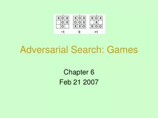
Example Game Tree for Tic-Tac-Toe • Tic-Tac-Toe also called Noughts and Crosses • 2-player, deterministic, alternating • The numbers on leaves indicate the utility values of terminal states from the point of view of the MAX
Minimax Search • A strategy/solution for optimal decisions • Examine the minimax value of each node in thegame tree • The is just the utility from the point of view of MAX • Assume two players (MAX and MIN) play optimally (infallibly) from the current node to the end of the game
Minimax Search • Example: a trivial 2-ply (one-move-deep) game • Perfect play for the deterministic, perfect-information game • MAX and MIN play optimally • Idea: choose the move to a position with highest minimax value = best achievable payoff against best play
Minimax Search: Example A vA=-∞ A vA=-∞ vA=-∞ A vB=3 B B vB=∞ B Terminal-Test 3 A A vA=-∞ vA=3 A vA=-∞ Backed up to root vB=3 vB=3 B B vB=3 B 8 12 8 3 12 12 3 3
Minimax Search: Example A vA=3 A vA=3 A vA=3 C vB=3 C vC=2 B vB=3 vC=2 B C vC=∞ vB=3 B 4 8 2 12 3 2 8 12 3 Backed up to root A vA=3 A vA=3 C vB=3 vC=2 C B vB=3 vC=2 B 4 6 8 2 12 3 4 6 8 2 12 3
Minimax Search: Example A vA=3 A vA=3 C C D vC=2 vD=∞ B vC=2 D vB=3 B vD=14 vB=3 4 6 8 2 12 3 4 6 14 8 2 12 3 A vA=3 A vA=3 C C vC=2 D vC=2 D B vD=2 vD=5 B vB=3 vB=3 4 6 4 6 8 2 12 5 2 5 8 2 12 3 3 14 14
Minimax Search: Example Backed up to root A vA=3 D C vD=2 vB=3 vC=2 B 5 2 14 4 6 8 2 12 3
Minimax Search • Algorithm For MAX Node For MIN Node
Minimax Search • Explanations of the Minmax Algorithm • A complete depth-first, recursive exploration of the game tree • The utility function is applied to each terminal state • The utility (min or max values) of internal tree nodes are calculated and then backed up through the tree as the recursion unwind • At the root, MAX chooses the move leading to the highest utility
Properties of Minimax Search • Is complete if tree is finite • Is optimal if the opponent acts optimally • Time complexity: O(bm) • m : the maximum depth of the tree • Space complexity: O(bm) or O(m) (when successors generated one at a time) For chess, b ≈ 35, m ≈ 100 for “reasonable” games I.e., exact solution is completely infeasible
Optimal Decisions in Multiplayer Games • Extend the minimax idea to multiplayer games • Replace the single value for each node with a vector of values • Alliances among players would be involved sometimes • E.g., A and B form an alliance to attack C If A and B are in an alliance
α-β Pruning • The problem with minimax search • The number of nodes to examine is exponential in thenumber of moves • α-β pruning • Applied to the minimax tree • Return the same moves as minimax would, but prune away branches that can’t possible influence the final decision • α: the value of best (highest-value) choice so far in search of MAX • β: the value of best (lowest-value) choice so far in search of MIN
α-β Pruning • Example A The subtree to be explored next should have a utility equal to or higher than 3 B
α-β Pruning • Example A C B The utility of this subtree will be no more than 2 (lower than current α), so the remaining children can be pruned
α-β Pruning • Example A C D B
α-β Pruning • Example A C B D
A C D B α-β Pruning • Example Can’t prune any successors of D at all because the worst successors of D have been generated first
α-β Pruning • The value of the root are independent of the value of the pruned leaves x and y
α-β Pruning • Algorithm For MAX Node Pruning: If one of its children has value larger than that of its best MIN predecessor node , return immediately. (?) For MIN Node Pruning: If one of its children has value lower than that of its best MAX predecessor node , return immediately. (?)
α-β Pruning (MAX) (MIN) Should examine some of n’sdescendant to reach the conclusion If m is better than n for Player (MAX), n will not be visited in play and can therefore be pruned
Properties of α-β Pruning • Pruning does not affect final result • The effectiveness of alpha-beta pruning is highly dependent on the order in which the successors are examined • Worthwhile to try to examine first the successors that are likely to be best • E.g., If the third successor “2” of node D has been generated first, the other two “14” and “5” can be pruned
Properties of α-β Pruning • If “perfect ordering” can be achieved • Time complexity: O(bm/2) • Effective branching factor becomes: b1/2 • Can double the depth of search within the time limit • If “random ordering” • Time complexity ≈O(b3m/4) for moderate b • Still have to search all the way to terminal statesfor at least a portion of the search space • The depth is usually not practical
Imperfect, Real-Time Decisions • Not feasible to search all the way to terminal statesin per move • When minimax search is adopted alone, or even whenalpha-beta pruning is additionally involved • Moves must be made in a reasonable amount of time • Shannon (1960) said • “…programs should cut off search earlier and apply a heuristic function to states in the search, effectively turning nonterminal nodes into terminal leaves…”
Imperfect, Real-Time Decisions • Minimax or alpha-beta altered in two ways • A heuristic evaluation functionEval is used to replace the utility function • Give an estimate of the expected utility of the game from a given position • Judge the value of a position • A cutoff test is used to replace the terminal test • Decide when to apply Eval • Turn nonterminal nodes into terminal leaves • A fixed depth limit is used (often add quiescence search)
Evaluation Functions • Criteria for good evaluation functions • Should order the terminal states in the same way as thetrue utility function • Avoid selecting suboptimal moves • Must not take too long to calculate • Time controls usually enforced • For nonterminal states, it should be strongly correlated with the actual chances of winning • Do not overestimate or underestimate too much • Chances here mean uncertainty, which is introduced by computational limits • A guess/prediction should be made
Evaluation Functions • Method 1: Most evaluation functions calculate and then combine various features of a state to give the estimation • E.g., the number of pawns possessed by each side in the chess game • Many states (with different board configurations) would have the same values of all features • States in the same category will win, draw, or lose proportionally/probabilistically • Too many categories to calculate the expected values for evaluation functions, and hence too much experience to estimate the probabilities win loss draw
Evaluation Functions • Method 2: Weighted linear function • Directly compute separate numerical contributions from each feature and then combine then to find the total value for a state • Assumptions: 1. features are independent on each other 2. values of features won’t change with time • The material value for each piece in the chess game • E.g., a pawn has a value of 1, a bishop/knight for 3, a rook for 5, a queen for 9 etc. The num. of each kind of piece on the board weights can be learned via machine learning techniques
Cutting Off Search • When to call the heuristic evaluation function in order to appropriately cut off the search if Cutoff-Test(state, depth) then return Eval(state) • Replace the “Terminal-Test” line in the algorithm • The amount of search is controlled by setting a fixed depth limit such that the time constraint will not be violated • Bookkeeping for the current node’s depth is needed Cutoff-Test(state, depth) • Return true for all depth greater than some fixed depth d, and vice versa • Return true for all terminal states • Iterative deepening search (IDS) can be applied here • Return the move selected by the deepest completed search
Cutting Off Search: Problems • Suppose when the program has searched to the depth limit and reached the following position (a) Black an advantage of a knight and two pawns and will win the game (b) Black will lose after white captures the queen • A more sophisticated cutoff test (for quiescence) is needed !
Cutting Off Search: Quiescence • A quiescent position is one which is unlikely to exhibit wild swings in value in the near future • Nonquiescent positions can be expanded further until quiescent positions are reached • Called quiescence search • Search for certain types of moves • E.g., search for “capture moves”
Deterministic Games in Practices • Checkers • 1994, the computer defeated the human world champion • Chess • 1997, Deep blue defeated the human world champion • Can seek 200 million positions per sec (almost 40 plies) • Othello • Computers are superior • Go • Humans are superior
Nondeterministic Games: Backgammon 西洋雙陸棋 • Games that combine luck and skill • Dice are rolled at the beginning of a player’s turn to determine the legal moves • E.g., Backgammon 1. Goal of the game: move all one’s pieces off the board 2. White moves clockwise toward 25 Black moves counterclockwise toward 0 3. A piece can move to any position unless there are multiple opponent pieces there 4. If the position to be move to has only one opponent, the opponent will be captured and restarted over 5. When one’s all pieces are in his home board, the pieces can be moved off the board … home board of black When white has rolled 6-5, it must choose among four legal moves: (5-10,5-11),(5-11,19-24),(5-10,10-16) and (5-11,11-16) home board of white
Nondeterministic Games: Backgammon • A game tree includes chance nodes MIN’s MAX’s If two dice used: - 21 distinct rolls - 15 ( ) with probabilities 1/18 - 6 ( ) with probabilities 1/36
Nondeterministic Games in General • Chance introduced by dice, card-shuffling • E.g., a simplified example with coin-flipping
Algorithm for Nondeterministic Games • Expectiminimax gives perfect play • Just like minimax, except chance nodes must be also handled
Pruning in Nondeterministic Game Trees • A version of α-β pruning is possible
Pruning in Nondeterministic Game Trees • A version of α-β pruning is possible
Pruning in Nondeterministic Game Trees • A version of α-β pruning is possible
Pruning in Nondeterministic Game Trees • A version of α-β pruning is possible
Pruning in Nondeterministic Game Trees • A version of α-β pruning is possible
Pruning in Nondeterministic Game Trees • A version of α-β pruning is possible
Pruning in Nondeterministic Game Trees • A version of α-β pruning is possible
Pruning in Nondeterministic Game Trees • A version of α-β pruning is possible 1.5