BSAD 6314 Multivariate Statistics

BSAD 6314 Multivariate Statistics

Major Goals: • Expand your repertoire of analytical options. • Choose appropriate techniques • Conduct analyses using available software. • Interpret findings • Know where to go for additional help.

What are Multivariate Stats? • Correlation 1 • Canonical Correlation • t test • One-way ANOVA • One way MANOVA IV • Multiple Regression • Canonical Correlation >1 • Factorial MANOVA • Factorial ANOVA 1 >1 DV

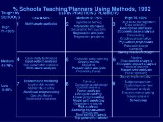
Hair Taxonomy Structure/ Independence Dependence Type of relationship # variables? Structure Single Rel.; Mult DVs One DV, Mult IVs Structure among cases/ people Mult Rel. IVs & DVs Structure among variables IV Cat. IV Cont. DV Cont. DV Cat. Factor Analysis Cluster Analysis SEM MANOVA Canon. Corr. Discrim; Log Regr Mult. Regr.

Matrices: • The math behind the statistics! • Two dimensional math represented in an array • People x Variables (OB/HR). • Organization x Variables (Strategy/OT).

The variables (V) can be continuous measures, categories represented by numbers, and transformations, products or combinations of other variables.

Nearly all statistical procedures—univariate and multivariate—are based on linear combinations. Understanding that basic fact has far-reaching implications for using statistical procedures to their fullest advantage. A linear combination (LC) is nothing more than a weighted sum of variables: LC = W1V1 + W2V2 + . . . + WKVK

LC = W1V1 + W2V2 + . . . + WKVK A very simple example is the total score on a questionnaire. The individual items on the questionnaire are the variables V1, V2, V3, etc. The weights are all set to a value of 1 (i.e., W1 = W2 = . . . Wk = 1). We call this unit weighting.

The items combined in a linear combination need not be variables. The items combined are often cases (e.g., people, groups, organizations). LC = W1P1 + W2P2 + . . . + WKPN A good example is the sample mean. In this case the weights are set to the reciprocal of the sample size (i.e., W1 = W2 = . . . Wk = 1/N).

Different statistical procedures derive the weights (W) in a linear combination to either maximize some desirable property (e.g., a correlation) or to minimize some undesirable property (e.g., error). The weights are sometimes assigned rather than derived (e.g., dummy, effect, and contrast codes) to produce linear combinations of particular interest.

Choice of Statistical Techniques • Research Purpose • Prediction, Explanation, Data Reduction • Number of IVs • Number of DVs • Measurement Scale • Continuous, categorical

Dependence/Prediction • Correlation • Regression • Multiple Regression • With nominal variables; Polynomials • Logistic regression/Dicriminant analysis • Canonical Correlation • MANOVA

The simplest possible inferential statistic-the bivariate correlation-involves just two variables. r

Continuous Continuous In its usual form, the correlation is calculated on variables that are continuous. r

Continuous Categorical When one of the variables is categorical, the calculation produces a point-biserial correlation. r

Categorical Categorical When both variables are categorical, the calculation produces a phi coefficient. r

Regression All forms of these correlations, however, can be recast as a linear combination: V2 predicted = A + BV1 r

OLS (ordinary least squares)Regression B and A can be chosen so that the sum of the squared deviations between V2 predicted and V2 are minimized. Solving for B and A using this rule also produces the maximum possible correlation between V1 and V2. r

Least Squared Error

The problem can be easily expanded to include more than one “predictor.” This is multiple regression: V4predicted = B1V1 + B2V2 + B3V3 + A Continuous Continuous R

The values for B1, B2, B3, and A are found by the least squares rule Continuous Continuous R

V1, V2, and V3 could be categorical contrast variables, perhaps coding the two main effects and the interaction from an experimental design. In that case, the multiple regression produces an analysis of variance. Categorical Continuous R

Or V2 might be the square of V1 and V3 might be the cube of V1. Then the multiple regression examines the polynomial trends. Continuous Continuous R

If the “outcome” variable is categorical, the basic nature of the analysis does not change. We still seek an “optimal” linear combination of V1, V2, and V3. Categorical “R”

Set A The basic multiple regression problem can be generalized to situations that involve more than one “outcome” variable. Set B R

Set A LCA = W1V1 + W2V2 + W3V3 + W4V4 + W5V5 + W6V6 Set B LCB = W7V7 + W8V8 + W9V9 + W10V10 + W11V11 + W12V12 RAB

Structure of Data • Goal is typically data reduction • How do the data “hang together? • Techniques include: • Factor analysis (the items) • Cluster analysis (the cases, people, organizations) • MDS (the objects)

Sometimes we are not interested in relations between sets of variables but instead focus on a single set and seek a linear combination that has desirable properties.

Or we might wonder how many “dimensions” underlie the 12 variables. These multiple dimensions also would be represented by linear combinations, perhaps constrained to be uncorrelated. These questions are addressed in principal components analysis and factor analysis.

A B C D

Sometimes we might shift the status of “people” and “variables” in our analysis. Our interest might be in whether a smaller number of dimensions or clusters might underlie the larger collection of people.

Approaches such as multidimensional scaling and cluster analysis can address such questions. These are conceptually similar to principal components analysis, but on a transposed matrix.

Structural Equation Modeling • Examines both structure of the data and predictive relationships simultaneously • Measurement model • Structural model

Structural equation models examine the relations among latent variables. Two kinds of linear combinations are needed. A1 A A2 D3 B1 B D D2 B2 D1 C1 C C2

The key idea is that the original data matrix can be transformed using linear combinations to provide useful ways to summarize the data and to test hypotheses about how the data are structured. Sometimes the linear combinations are of variables and sometimes they are of people.

Once a linear combination is created, we also need to know something about its variability. Everything we need to know about the variability of a linear combination is contained in the variance-covariance matrix of the original variables (S). The weights that are applied to create a linear combination can also be applied to S to get the variance of that LC. s12r12 = _______ (s21s22)½

BSAD 6314 Multivariate Statistics