Chapter 9 Calculus of variations

1. Mathematical methods in the physical sciences 3rd edition Mary L. Boas Chapter 9 Calculus of variations Lecture 10 Euler equation

2. 1. Introduction - Geodesic: a curve for a shortest distance between two points along a surface 1) On a plane, a straight line 2) On a sphere, a circle with a center identical to the sphere 3) On an arbitrary surface, ???  In this case, we can use the calculus of the variation. cf. Because the geodesic is the shortest value, finding the geodesic is relevant to finding the max. or min. values.

3. - In the ordinary calculus with f(x), how can you find the max. or min? (or how can you make the quantity stationary) First, obtain the first derivative of f(x), and find the stationary points. : Stationary point to make f’(x)=0. f(x) becomes Max. and Min. points and more. cf. But, we do not know if a given stationary point is a Max, Min, or a point of the inflection with a horizontal tangent.

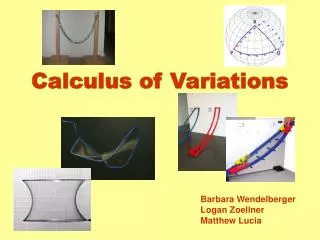
4. - What is the quantity which we want to make stationary in this chapter? Ex. 1) shortest distance Ex. 2) brachistochrone problem: brachistos=shortest, chronos=time e.g., In what shape should you bend a wire joining two given points so that a bead will slide down from one point to the other in the shortest time? We must minimize “time”. ds : element of arc length, v=ds/dt : velocity

5. Ex. 3) a soap film suspended between two rings What is the shape of the surface? The answer is the shape to minimize the surface area. Other examples - chain suspended between two points hangs so that its center of gravity is as low as possible. - Fermat’s principle in optics. (light traveling between two given points follows the path requiring the least time.

6. 2. Euler equation 1) Geodesic on a plane We call this y(x) ‘extremal’. We define a completely arbitrary function passing two points.

7. Then, our problem is to make I() take its min. when  = 0.

8. - first term is zero because (x1)= (x2)=0. - (x) is an arbitrary function. In order for the second term to be zero, **From this, y(x) (geodesic on a plane) is a straight line.

9. 2) Generalization For arbitrary ,

10. Example geodesic on a plane

11. Mathematical methods in the physical sciences 3rd edition Mary L. Boas Chapter 9 Calculus of variations Lecture 11 Application of Euler equation

12. 3. Using the Euler equation 1) Other variables Note. 1. The first derivative is with respect to the integration variable in the integral. 2. The partial derivatives are with respect to the other variables and its derivatives.

13. Example 1. Find the path followed by a light ray if n (refractive index) is prop. to r-2 (polar coord.).

15. 2) First integrals of the Euler equation In this case, we can integrate the Euler equation once. Such a equation (F/ y’) is called a first integral of the Euler equation.

16. p2 curve, y(x) p1 revolving the curve about x-axis Example 2. Find the curve so that the surface area of revolution is minimized. a surface of revolution

17. ‘catenary line (현수선)’

18. - Like the above, if F(y,y’) does not have the independent variable x, we had better change to y as integration variable. Example 3.

19. Example 4. Find the geodesics on the cone z^2=8(x^2+y^2) using the cylindrical coordinate.

21. 4. Brachistochrone problem: cycloids A bead slides along a curve from (x1,y1)=(0.0) to (x2,y2). Find the curve to minimize the during time. The sum of two energies is zero initially and therefore zero at any time and position. reference ‘gravity’

22. The integral we want to minimize is

23. c’=0 for (x1, y1) = (0,0) “This is the equation of a cycloid.”

24. - Cycloid A circle (radius a) rolls along x-axis. It start at origin O. Place a mark on the circle at O. As the circle rolls, the mark traces out a cycloid. “trace of a mark on the circle when the circle rolls.”

25. - Parametric equation of a cycloid When a circle rolled a little, ‘parametric equation of a cycloid’

26. “parametric equation of brachistochrone or parametric equation of cycloid.”

27. - Cycloids differ from each other only in size, not in shape. - Rather surprisingly, when a bead slides from origin to P3 in the least time, it goes down to P2 and backs up to P3 !! At P2, x/y = /2. For P1, x/y < /2. For P3, x/y > /2.

28. Mathematical methods in the physical sciences 2nd edition Mary L. Boas Chapter 9 Calculus of variations Lecture 12 Lagrange’s equations

29. 5. Several dependent variables; Lagrange’s equation - Necessary condition for a minimum point in ordinary calculus, for an one-variable function z=z(x), dz/dx=0, for a two-variable function z=z(x, y), z/x=0 and z/y=0. - The similar idea is applied to Euler equation. When for F=F(x, y, z, dy/dx, dz/dx) we find two curves y(x) and z(x) to minimize I =  F dx, we need two Euler equations.

30. It is a very important application to mechanics ; Lagrangian based on Hamilton’s principle - Lagrangian: L = T – V where T : kinetic energy, V : potential energy - Hamilton’s principle: any particle or system of particles always moves in such a way that I =  L dt is stationary. In this case, Euler equation is called Lagrange’s equation.

31. Example 1. Equation of motion of a single particle moving (near the earth) under gravity. (three dimensional motion)

32. - In some cases, it would be simpler to use elementary method from Newton’s equation. However, in some cases with many variables it would be much simpler to use Lagrange’ equation, because we treat one scalar function, Lagrangian L = T – V.

33. Example 2. Equation of motion in terms of polar coordinate variable r, . Coriolis acceleration centripetal v^2/r

34. Example 3. m1 moves on the cone. (spherical coord. , , ) m2 is joined to m1 and move vertically up and down. (z-component) Here, the cone ( =30) is a constraint for motion. Using the above,

36. cf. Rolling disk

37. cf. Atwood’s machine I

39. cf. Atwood’s machine II

40. cf. Swing atwood’s machine

41. cf. Double pendulum

42. cf. Prob. 19

43. 6. Isoperimetric problems Ex. To find a curve to make largest area ( y dx = Max.) with a given length ( ds = l) cf. Lagrange multiplier (Max. or min. (stationary point) problem with a constraint) By using the Lagrange multiplier method, - Good news: Sometimes we do not need to find .

44. x1 x2 Example 1. Find the shape of the curve of constant length joining two points x_1 and x_2 on the x-axis which, with the x axis, encloses the largest area. The curve length is fixed. (l > x2-x1)

46. 7. Variation notation -  : differentiation with respect to . just like the symbol d in a differential except that , not x, is a differential variable.

47. - The meanings of two statement are the same. (a) I is stationary; that is, dI/d=0 at =0. (b) The variation of I is zero; that is, I=0

48. H. W (Due 13th of Nov.) Chap. 9 2-1 3-4,5 5-4 (G1), 5(G2), 9(G3) 6-1, 2(G4)

49. Problem 5-4 Use Lagrange’s equations to find the equation of motion of a simple pendulum. 5-5. Find the equation of motion of a particle moving along the x axis if the potential energy is V=(1/2)kx^2. 5-9 A mass m moves without friction on the surface of the corner r = z under gravity acting in the negative z direction. Find the Lagrangian and Lagrange’s equation in terms of r, . 6-2 The plane area between the curve and a straight line joining the points is a maximum.