Download
1 / 96
1.02k likes | 1.6k Vues
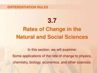
DIFFERENTIATION RULES. 3.7 Rates of Change in the Natural and Social Sciences. In this section, we will examine: Some applications of the rate of change to physics, chemistry, biology, economics, and other sciences. RATES OF CHANGE.

E N D
DIFFERENTIATION RULES 3.7Rates of Change in the Natural and Social Sciences In this section, we will examine: Some applications of the rate of change to physics, chemistry, biology, economics, and other sciences.
RATES OF CHANGE • Let’s recall from Section 2.7 the basic idea behind rates of change. • If x changes from x1 to x2, then the change in xis ∆x = x2 – x1 • Thecorresponding change in y is ∆y = f(x2) – f(x1)
AVERAGE RATE • The difference quotient • is the average rate of change of y with respect to x over the interval [x1, x2]. • It can be interpreted as the slope of the secant line PQ.
INSTANTANEOUS RATE • Its limit as ∆x → 0 is the derivative f’(x1). • This can therefore be interpreted as the instantaneous rate of change of y with respect to x or the slope of the tangent line at P(x1,f(x1)).
RATES OF CHANGE • Using Leibniz notation, we write the process in the form
RATES OF CHANGE • Whenever the function y = f(x) has a specific interpretation in one of the sciences, its derivative will have a specific interpretation as a rate of change. • As we discussed in Section 2.7, the units for dy/dxare the units for y divided by the units for x.
NATURAL AND SOCIAL SCIENCES • We now look at some of these interpretations in the natural and social sciences.
PHYSICS • Let s = f(t) be the position function of a particle moving in a straight line. Then, • ∆s/∆t represents the average velocity over a time period ∆t • v = ds/dt represents the instantaneous velocity (velocity is the rate of change of displacement with respect to time) • The instantaneous rate of change of velocity with respect to time is acceleration: a(t) = v’(t) = s’’(t)
PHYSICS Example 1 • The position of a particle is given by the equation s = f(t) = t3 – 6t2 + 9t where t is measured in seconds and s in meters. • Find the velocity at time t. • What is the velocity after 2 s? After 4 s? • When is the particle at rest?
PHYSICS Example 1 • When is the particle moving forward (that is, in the positive direction)? • Draw a diagram to represent the motion of the particle. • Find the total distance traveled by the particle during the first five seconds.
PHYSICS Example 1 • Find the acceleration at time t and after 4 s. • Graph the position, velocity, and acceleration functions for 0 ≤ t ≤ 5. • When is the particle speeding up? When is it slowing down?
PHYSICS Example 1 a • The velocity function is the derivative of the position function. s = f(t) = t3 – 6t2 + 9t • v(t) = ds/dt = 3t2 – 12t + 9
PHYSICS Example 1 b • The velocity after 2 s means the instantaneous velocity when t = 2, that is, • The velocity after 4 s is:
PHYSICS Example 1 c • The particle is at rest when v(t) = 0, that is, • 3t2 - 12t + 9 = 3(t2 - 4t + 3) = 3(t - 1)(t - 3) = 0 • This is true when t = 1 or t = 3. • Thus, the particle is at rest after 1 s and after 3 s.
PHYSICS Example 1 d • The particle moves in the positive direction when v(t) > 0, that is, • 3t2 – 12t + 9 = 3(t – 1)(t – 3) > 0 • This inequality is true when both factors are positive (t > 3) or when both factors are negative (t < 1). • Thus the particle moves in the positive direction in the time intervals t < 1 and t > 3. • It moves backward (in the negative direction) when 1 < t < 3.
PHYSICS Example 1 e • Using the information from (d), we make a schematic sketch of the motion of the particle back and forth along a line (the s -axis).
PHYSICS Example 1 f • Due to what we learned in (d) and (e), we need to calculate the distances traveled during the time intervals [0, 1], [1, 3], and [3, 5] separately.
PHYSICS Example 1 f • The distance traveled in the first second is: • |f(1) – f(0)| = |4 – 0| = 4 m • From t = 1 to t = 3, it is: • |f(3) – f(1)| = |0 – 4| = 4 m • From t = 3 to t = 5, it is: • |f(5) – f(3)| = |20 – 0| = 20 m • The total distance is 4 + 4 + 20 = 28 m
PHYSICS Example 1 g • The acceleration is the derivative of the velocity function:
PHYSICS Example 1 h • The figure shows the graphs of s, v, and a.
PHYSICS Example 1 i • The particle speeds up when the velocity is positive and increasing (v and a are both positive) and when the velocity is negative and decreasing (v and a are both negative). • In other words, the particle speeds up when the velocity and acceleration have the same sign. • The particle is pushed in the same direction it is moving.
PHYSICS Example 1 i • From the figure, we see that this happens when 1 < t < 2 and when t > 3.
PHYSICS Example 1 i • The particle slows down when v and a have opposite signs—that is, when 0 ≤ t < 1 and when 2 < t < 3.
PHYSICS Example 1 i • This figure summarizes the motion of the particle.
PHYSICS Example 2 • If a rod or piece of wire is homogeneous, then its linear density is uniform and is defined as the mass per unit length (ρ = m/l) and measured in kilograms per meter.
PHYSICS Example 2 • However, suppose that the rod is not homogeneous but that its mass measured from its left end to a point xis m = f(x).
PHYSICS Example 2 • The mass of the part of the rod that lies between x = x1 and x = x2 is given by ∆m = f(x2) – f(x1)
PHYSICS Example 2 • So, the average density of that part is:
PHYSICS Example 2 • If we now let ∆x → 0 (that is, x2 → x1), we are computing the average density over smaller and smaller intervals.
LINEAR DENSITY • The linear density ρ at x1 is the limit of these average densities as ∆x → 0. • That is, the linear density is the rate of change of mass with respect to length.
LINEAR DENSITY Example 2 • Symbolically, • Thus, the linear density of the rod is the derivative of mass with respect to length.
PHYSICS Example 2 • For instance, if m = f(x) = , where x is measured in meters and m in kilograms, then the average density of the part of the rod given by 1≤ x ≤ 1.2 is:
PHYSICS Example 2 • The density right at x = 1 is:
CHEMISTRY Example 4 • A chemical reaction results in the formation of one or more substances (products) from one or more starting materials (reactants). • For instance, the ‘equation’ 2H2 + O2→ 2H2O indicates that two molecules of hydrogen and one molecule of oxygen form two molecules of water.
CONCENTRATION Example 4 • Let’s consider the reaction A + B → C where A and B are the reactants and C is the product. • The concentrationof a reactant A is the number of moles (6.022 X 10²³ molecules) per liter and is denoted by [A]. • The concentration varies during a reaction. • So, [A], [B], and [C] are all functions of time (t).
AVERAGE RATE Example 4 • The average rate of reaction of the product C over a time interval t1≤t≤t2 is:
INSTANTANEOUS RATE Example 4 • However, chemists are more interested in the instantaneous rate of reaction. • This is obtained by taking the limit of the average rate of reaction as the time interval ∆tapproaches 0: rate of reaction =
PRODUCT CONCENTRATION Example 4 • Since the concentration of the product increases as the reaction proceeds, the derivative d[C]/dt will be positive. • So, the rate of reaction of C is positive.
REACTANT CONCENTRATION Example 4 • However, the concentrations of the reactants decrease during the reaction. • So, to make the rates of reaction of A and B positive numbers, we put minus signs in front of the derivatives d[A]/dt and d[B]/dt.
CHEMISTRY Example 4 • Since [A] and [B] each decrease at the same rate that [C] increases, we have:
CHEMISTRY Example 4 • More generally, it turns out that for a reaction of the form • aA + bB →cC + dD • we have
CHEMISTRY Example 4 • The rate of reaction can be determined from data and graphical methods. • In some cases, there are explicit formulas for the concentrations as functions of time—which enable us to compute the rate of reaction.
ECONOMICS Example 8 • Suppose C(x) is the total cost that a company incurs in producing x units of a certain commodity. • The function C is called a cost function.
AVERAGE RATE Example 8 • If the number of items produced is increased from x1 to x2, then the additional cost is ∆C = C(x2) - C(x1) and the average rate of change of the cost is:
MARGINAL COST Example 8 • The limit of this quantity as ∆x → 0, that is, the instantaneous rate of change of cost with respect to the number of items produced, is called the marginal costby economists:
ECONOMICS Example 8 • As x often takes on only integer values, it may not make literal sense to let ∆x approach 0. • However, we can always replace C(x) by a smooth approximating function—as in Example 6.
ECONOMICS Example 8 • Taking ∆x = 1 and n large (so that ∆xis small compared to n), we have: • C’(n) ≈ C(n + 1) – C(n) • Thus, the marginal cost of producing n units is approximately equal to the cost of producing one more unit [the (n + 1)st unit].
ECONOMICS Example 8 • It is often appropriate to represent a total cost function by a polynomial • C(x) = a + bx + cx2 + dx3 • where a represents the overhead cost (rent, heat, and maintenance) and the other terms represent the cost of raw materials, labor, and so on.
ECONOMICS Example 8 • The cost of raw materials may be proportional to x. • However,labor costs might depend partly on higher powers of x because of overtime costs and inefficiencies involved in large-scale operations.
ECONOMICS Example 8 • For instance, suppose a company has estimated that the cost (in dollars) of producing x items is: • C(x) = 10,000 + 5x + 0.01x2 • Then, the marginal cost function is:C’(x) = 5 + 0.02x