Download

1 / 16
240 likes | 725 Vues
GAME THEORY AND INDUSTRIAL ECONOMICS (ORGANIZATION). FIRMS’ STRATEGIC BEHAVIOUR Strategic interaction among economic agents (a sort of externality: the action of firm A affects the profits of firm B)

E N D
GAME THEORY AND INDUSTRIAL ECONOMICS (ORGANIZATION) • FIRMS’ STRATEGIC BEHAVIOUR • Strategic interaction among economic agents (a sort of externality: the action of firm A affects the profits of firm B) • OLIGOPOLY: it is not (necessarily) characterised by the presence of a few – large – firms but it emerges when there is interdependence among firms “Except where monopoly is assumed and the possibility of entry is assumed away, theoretical research in industrial economics today employs the tools of non-cooperative game theory. […] It is then assumed that the observed behaviour will correspond to a Nash equilibrium of the specified game, a situation in which each firm’s strategy (…) is a best response to the strategies of its rivals”. (R. Schmalensee, Industrial economics: an overview, Economic Journal, 1988, p. 645)
Basic elements of a game • Players: in our case, firms. Sometimes, to insert an element of exogenous uncertainty, a player called “Nature” appears in the game • Rules of the game: possible actions or moves but also, and most importantly, the information available at the point of each move • Strategies: single actions or sequences of actions (choices of output quantity, price, product quality, R&D expenditures, …) • Pure strategies: played with certainty (to fix a price high or low) • Mixed strategies: played with a given probability (to fix a price high with a probability of 0.7 and a price low with a probability of 0.3) • Payoffs: the players’ objectives (i.e. profits) • Form of the game: normal or strategic (matrix) and extensive (tree)
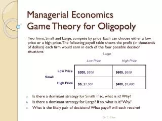
Oligopoly Pricing Game Normal form Nash equilibrium = Low-Low (Pareto inferior)
Extensive form Pepsi High Low Coke a b High Low High Low (1500,1500) (500,1700) (1700,500) (1000,1000)
TYPES OF INFORMATION • Complete information: all the players know all the elements of the game (number of players, strategies, payoffs, etc.) • Incomplete information: the game begins with a move of “Nature” which makes unknown an element of the game In sequential (non simultaneous) games (where one player moves first): • Perfect information: each player knows the branch of the game tree in which is located (i.e. observes the moves of other players) • Imperfect information (opposite) • In presence of imperfect information, the outcome of a simultaneous static game (normal form) is identical to that of a sequential game (extensive form)
TYPES OF GAMES • Cooperative games (presence of binding agreements among players) • Non cooperative games (variable or zero-sum games) • Our focus will be on non cooperative games with variable sum • We shall begin with static, “one-shot”, non-cooperative games • Then, we shall move to other games in which “time” is included in the form of a sequence of decision making • Repeated games (not treated in our lectures) • Multiple-stage games: for instance a two-stage game in which in the first stage the firms chose the product quality and in the second stage chose (i.e. compete in) prices • Solution by backward induction: find the equilibrium of the second stage and use it to find the first stage equilibrium • The latter games are widely used in Industrial Organization
NON-COOPERATIVE GAMES: NASH EQUILIBRIUM • John Nash (1950) proved the existence of an equilibrium point in non-cooperative games • Nash theorem: every game with a finite number of players and strategies has, at least, one equilibrium (in pure or mixed strategies) • Each player chooses the “best-response” strategy (that maximising her/his payoff) to other players’ strategies. So, intuitively, if every one is making the best response to everyone else, no player will change her/his strategy • Problem: multiple Nash equilibria
Sequential game (with perfect information) Janet Theater Football Mark a b Theater Football Theater Football (3, 2) (1, 1) (1, 1) (2, 3)
NASH EQUILIBRIUM IN OLIGOPOLY • In oligopoly, the Nash equilibrium coincides with that of: • Cournot, when the strategies are based on output quantities (Cournot-Nash equilibrium): LONG-RUN CHOICE • Bertrand, when the strategies are based on prices (Bertrand-Nash equilibrium): SHORT-RUN CHOICE
Duopoly models • Πi(ai,aj) profit function twice continuously differentiable in the actions; ai= action of firm i (price or quantity) • A pair of feasible actions is a Nash equilibrium if Πi(a*i,a*j) ≥Πi(ai,a*j) • F.O.C. Πii(ai,aj)=0 (where Πii= ∂Πi/∂ai) • From this we get the reaction functions (best response functions) of the two firms: Ri(aj) is the best response of firm i when firm j chooses aj • Nash equilibrium (solve the system of two equations with two unknowns): a*i=Ri(a*j) and a*j=Rj(a*i)
COURNOT MODEL • Original duopoly model by Antoine Augustin Cournot (1838): Researches into the mathematical principles of the theory of wealth (Chapter VII “Of the competition of producers”). • Two “proprietors” of water springs with identical quality and zero production costs. Hypotheses: product homogeneity; equal and constant marginal costs = zero production costs. • Each producer is aware that the rival's quantity decision will also affect the price he faces and thus his profits. Consequently, each producer chooses a quantity that maximizes his profits subject to the quantity chosen by the rival.
The above is the concept of “reaction function”. The symmetric equilibrium quantities can be drawn as the intersection of the reaction curves of the two producers. Given the quantities, one can get the equilibrium price and, then, the symmetric producers’ profits • Comparing solutions, Cournot notes that under duopoly, the price is lower and the total quantity produced greater than under monopoly. In the subsequent chapter, he shows that as the number of producers increases, the quantity becomes greater and the price lower • This is the Cournot paradigm for antitrust policy (which, however, holds only in presence of constant returns to scale)
BERTRAND MODEL • In 1883 Joseph Bertrand published a review of the Cournot’s book (which, up to then, had been neglected by economists). He radically criticised the Cournot duopoly model for being based on the choice of quantities rather than prices • If the product is homogenous and two firms with identical linear cost functions choose prices, the price competition will led to a perfectly competitive equilibrium= price equal to marginal cost and zero profits • This is the well known Bertrand paradox, which can be “solved” in many ways (see below)
PRICE GAME WITH HOMOGENEOUS PRODUCTS (BETRAND GAME) ΠM = monopoly profits Nash equilibrium = Low-Low = zero profits
AVOIDING BERTRAND PARADOX • Capacity constraint. Originally introduced by Edgeworth (1897). Reprised by Kreps and Scheinkman (1983) Quantity pre-commitment and Bertrand competition yeld Cournot outcomes, BJoE (two-stage game: in the first stage firms choose productive capacity and in the second compete in prices). • Product differentiation. Hotelling model (1929) of horizontal differentiation revisited by d’Aspremont, Gabszewicz and Thisse (1979) On Hotelling’s stability in competition, Econometrica [two-stage game: in the first firms choose the location in the space of characteristics and in the second compete in prices]. Vertical differentiationmodel of Shaked and Sutton (1982) Relaxing price competition through product differentiation REc&St [three-stage game]. • Repeated game.Under given conditions the collusion is an equilibrium (Folk Theorem) and the two firms gain half of the monopoly profit.

![READ [PDF] Industrial Organization: Theory and Practice (The Pearson Series in Economics)](https://cdn7.slideserve.com/12565050/slide1-dt.jpg)
![[PDF] DOWNLOAD Industrial Organization: Theory and Applications](https://cdn7.slideserve.com/12596906/slide1-dt.jpg)
![[PDF READ ONLINE] Industrial Organization: Theory and Applications](https://cdn7.slideserve.com/12623578/pdf-read-online-industrial-organization-theory-dt.jpg)