The distance from dS to P is

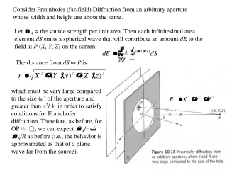
1. Consider Fraunhofer (far-field) Diffraction from an arbitrary aperture whose width and height are about the same. Let A = the source strength per unit area. Then each infinitesimal area element dS emits a spherical wave that will contribute an amount dE to the field at P (X, Y, Z) on the screen The distance from dS to P is which must be very large compared to the size (a) of the aperture and greater than a2/ in order to satisfy conditions for Fraunhofer diffraction. Therefore, as before, for OP  , we can expect A/r  A/R as before (i.e., the behavior is approximated as that of a plane wave far from the source).

2. Fig. 10.19 A rectangular aperture. At point P (X, Y), the complex field is calculated as follows:

3. For x, y << R, we can approximate r as follows: Thus, for the specific geometry of the rectangular aperture:

4. Therefore, the resulting complex field at point P on the screen for a rectangular aperture having area A = ab is given by where I(0) is the intensity at the center of the screen at point P0 (Y = 0, Z = 0). A typical far-field diffraction pattern is shown in Fig. 10.20. Note that when  = 0 or  = 0, we get the familiar single slit pattern. The approximate locations of the secondary maxima along the -axis (which is the Y- axis when  = 0 or Z = 0) is given by m  3/2, 5/2, 7/2... Since sin  = 1 at these maxima, the relative irradiances along the -axis are approximated as where m  3/2, 5/2, 7/2... 

5. Square aperture in which a = b. where m= m  3/2, 5/2, 7/2... are the positions of the secondary maxima and Distribution of irradiance, I(Y,Z) Distribution of electric field, E(Y,Z)  (Z)  (Y)

6. A very important aperture shape is the circular hole, as this involves the natural symmetry for lenses. Such a symmetry suggests the need for cylindrical coordinates: We are calculating the field E on the screen  as a function of the screen’s radial coordinate q. Fig. 10.21 Circular Aperture Geometry

7. The circular shape of the aperture results in complete axial symmetry. Therefore, the solution must be independent of . Therefore, we are permitted to set  = 0. We are therefore led to evaluate the integral: where J0(u) is the Bessel function (BF) of order zero. More generally the BF of order m, Jm(u), is represented by the following integral: Bessel functions are slowly decreasing oscillatory functions very common in mathematical physics. Fig. 10.22 Therefore the field is expressed as

8. Another important property of the Bessel Function is the recurrence relation that connects BFs of consecutive orders:

9. We can express the field, using the recurrence relation, as Therefore, the irradiance at point P on the screen is It is useful to examine the series representation of the Bessel Functions:

10. Consider the limit near x = 0 : Therefore, the irradiance at P0 when q = 0 is and the Irradiance becomes (Fig. 10.21) We usually express the irradiance as a function of the angular deviation  from the central maximum at point P0. The large central maximum is called the Airy Disk, which is surrounded by the first dark ring corresponding to the first zero of J1(u). J1(u) = 0 when u = 3.83 or kaq1/R = kasin1= 3.83.

11. D = 2a is the diameter of the circular hole Note that ~84% of the light is contained in the Airy Disk (i.e. 0  kasin  3.83) Airy Disk Airy Disk

12. Airy Rings with different hole diameters Suppose that the aperture is a lens which focuses light on a screen: D = 0.5 mm screen Converging lens Entrance Pupil (Aperture) f D = 1.0 mm Airy Disk D which gives the radius of the Airy disk on the screen.

13. Analysis of overlapping images using Airy rings Rays arriving from two stars and striking a lens Suppose that we image two equal irradiance point sources (e.g., stars) through the objective lens of a telescope. The angular half-width of each image point is q1/f = sin    . If the angular separation of the stars is  and  >>  the images of the stars will be distinct and well resolved. Fig. 10.24 Overlapping Images

14. Rayleigh’s criterion for the minimum resolvable angular separation or angular limit of resolution Half-angle of an airy disk: f Rays from two stars If the stars are sufficiently close in angle so that the center of the Airy disk of star 1 falls on the first minimum (dark ring) of the Airy pattern of star 2, we can say that the two stars are just barely resolved. In this case, we have 1 = ( )min = q1/f  1.22  / D  (l)min 1.22 f/D . This is Rayleigh’s criterion for angular or spatial resolution. )l(min Fig. 10.25

15. Another criterion for resolving two objects has been proposed by C. Sparrow. At the Rayleigh limit there is a central minimum between adjacent peaks. Further decrease in the distance between two point sources will cause this minimum (dip) to disappear such that Sp The resultant maximum will therefore have a broad flat top when the distance between the peaks is r = Sp, and serves as the Sparrow criterion for resolving two point objects.

16. Diffraction Gratings Transmission Grating is made by scratching rulings or notches onto a clear flat plate of glass. Each notch serves as a source of scattering that affects radiating secondary sources, in much the same way as for a multiple-slit diffraction array. When the phase conditions are met through OPD =  = m, constructive interference is observed. Oblique incidence (i > 0) from the geometry. m = 0 (zeroth order), m = 1 (first order), m = 2 (second order), m = 3 (third order)

17. The diffraction grating can also be constructed as a reflection grating. The principals and conditions for constructive interference are the same as that for a transmission grating. Most commercial gratings for spectroscopy are constructed with a Blaze angle  to control the efficiency of diffraction for a particular  and order m.

18. Controlling the irradiance distribution of diffracted orders using a Blazed grating. Consider the situation such that: i = 0 so m = 0, 0 = 0. For specular reflection i - r = 2 and so most of the diffracted irradiance is concentrated near r = -2. This will correspond to a particular non-zero order in which m = -2 and asin(-2) = m. Most of the incident light undergoes specular reflection, similar to a plane mirror, and this occurs when i = m and m = 0 for the zeroth order beam. The problem is that most of the irradiance is wasted for the purpose of spectroscopy. It is possible to shift the reflected energy distribution into a higher order (m = 1) in which m depends on . It is possible to change the distribution of the specular reflection by changing the blaze angle  so that the first order diffraction is optimized for a particular range of wavelengths.

19. Schematic from the Fluorescence Group, University of California, Santa Barbara, USA

20. Monochromators with micrometer adjustable entrance and exit slit widths • Exit slit determines spectral resolution of the instrument • Resolution is determined by the product of the monochromator linear dispersion (nm/mm) and the slit width • Monochromator resolution depends on the grating pitch and the (focal) length of the monochromator • For PTI monochromator with 1200 groove/mm grating the reciprocal linear dispersion is 4 nm/mm. • 1 turn of the slit micrometer = 0.5 mm slit opening   = 2 nm spectral resolution. Note that since E = h = hc/  E = (-hc/2)  Example of luminescence spectra measured with a grating monochromator on the left for GaN/InGaN multiple quantum well (QW) samples. The maximum spectral resolution is obtained for the narrowest slit widths. Sit widths narrow (top) and wide (bottom)

21. Cathodoluminescence (CL) - Light emitted by the injection of high-energy electrons. Photomultiplier Tube (PMT) or Ge p-i-n detector From Prof. Rich’s Laboratory for Optical Studies of Quantum Nanostructures

22. Fresnel (Near-Field) Diffraction The basic idea is to start again with the Huygen’s-Fresnel principle for secondary spherical wave propagation. At any instant, every point on the primary wavefront is envisioned as a continuous emitter of spherical secondary wavelets. However, no reverse wave traveling back toward the source is detected experimentally. Therefore, in order to introduce a realistic radiation pattern of secondary emitters, we introduce the inclination factor, K() = (1+cos)/2 which describes the directionality of secondary emissions. K(0) = 1 and K() = 0.

23. A rectangular aperture in the near-field (Fresnel Diffraction) The monochromatic point source S and the point P on a screen are placed sufficiently close to the aperture where far-field conditions are no longer applicable. Consider a point A in the aperture whose coordinates are (y,z). The location of the origin O is determined by a perpendicular line from the source S to the aperture . The field contributions at P from the secondary sources on dS (area element at point A) is given by where 0 is the source strength at S, A is the secondary wavelet source strength per area, and A = 0 is obtained from the Huygen’s-Fresnel formalism.

24. In the case where the dimensions of the aperture are small compared to  and r, we can assume primarily forward propagation in the secondary spherical waves so that K()  1 and 1/r  1/0r0. Also, from the figure the geometry yields: Expand both terms in a binomial series for small y and z: Note that this approximation contains quadratic terms that appear in the phase whereas the Fraunhofer approximation contains only linear terms. Thus, we can expect a greater sensitivity in the phase of the cosine for this near-field treatment. The complex field at point P on the screen is therefore:

25. This is the unobstructed disturbance at P. where A(w) and C(w) are called Fresnel Integrals; note that both are odd functions of w.

26. Very often, we work in the limit of incoming plane-waves striking the aperture. For example, a laser beam could strike the aperture. In this limit we let the radius from the source to the aperture 0  . This results in an immediate simplification for the change of variables: Cornu Spiral Elegant geometrical description of the Fresnel Integrals (Fig. 10.50).

27. Fig. 10.50 The Cornu Spiral for a graphical representation of the Fresnel integrals. C(w) A(w)

28. w A(w) C(w) w A(w) C(w) A(w) C(w) A(w) C(w)

29. Therefore, values of w in B(w) correspond to arc length on the Cornu spiral. z (1 mm, 1 mm) (-1 mm, 1 mm) Consider a 2-mm square aperture hole: (y2, z2) (y1, z2) We are given that  = 500 nm, r0 = 4 m, plane wave approx. is valid. Find the irradiance at a point P on the screen along the axis x, directly behind the center of the aperture. y O (y2, z1) (y1, z1) (1 mm, -1 mm) (-1 mm, -1 mm) r0 P

30. Notice that there is an increase of the irradiance at the center point P on the screen by 256% relative to the unobstructed intensity due to a redistribution of the energy. z (-0.9 mm, 1 mm) (1.1 mm, 1 mm) In order to find the irradiance 0.1 mm to the left of center, move the aperture to the right relative to the OP line. While y1 and y2 are shifted, z1 and z2 remain unchanged. Then we have u2 = 1.1, u1 = -0.9, v2 = 1.0, v1 = -1.0. (y1, z2) (y2, z2) y (y2, z1) (y1, z1) (1.1 mm, -1 mm) (-0.9 mm, -1 mm) r0

31. The decrease in the irradiance (2.485I0 < 2.56I0) for a small 0.1 mm shift to the left (or right) of center on the screen shows that the center position is a relative maximum (see Cornu spiral on the next slide). Note that if the aperture is completely opened: which must equal to the unobstructed intensity as a check.

32. 1.1 C(w) A(w) -0.9 The decrease in the complex vector length from the position of the central peak shows that the central position is a maximum.

33. We can apply this formalism for Fresnel diffraction by a long narrow slit in which b = z1 – z2 = slit width and let v = v2 – v1 which is a string of length v lying along the Cornu spiral (next slide).

34. Suppose that v = 2. At point P, opposite point O in the aperture, the aperture and the screen are centered symmetrically and the string is centered at point Os. If the aperture is moved up or down, the arc length of the string remains constant, but the length of the vector B12(v) changes, as before. It should be apparent that the length of B12 (and the intensity at point P on the screen) will oscillate as the string slides around one of the spirals, which is equivalent to the slit moving up or down with respect to a reference point on the screen, as shown in the previous slide.

35. It is also possible to visualize a clear minimum at the center of the near field diffraction pattern on the screen by considering the an arc-length of w = 3.5. Any change in the slit position will give and increase in B12 and therefore an increase in irradiance. It is apparent that the slit width has a marked effect on whether the central position is a maximum or local minimum. Also note the oscillation in irradiance for positions beyond the width of the slit in both cases.