Download

1 / 33
330 likes | 375 Vues
Understand the Markowitz Model and Efficient Frontier to optimize your portfolio for risk and return. Learn about CAPM and risk-free assets to make informed investment decisions.

E N D
Chapter 5 CAPITAL MARKET THEORY
MARKOWITZ MODEL AND EFFICIENT FRONTIER • The Markowitz Model of portfolio analysis generates an efficient frontier, which is a set of efficient portfolios. • Efficient portfolio is that portfolio which has no alternative with • The same expected return of portfolio and lower standard deviation of portfolio • The same standard deviation of portfolio and higher expected return of portfolio • A higher expected return of portfolio and lower standard deviation
EFFICIENT FRONTIER FOR A TWO-SECURITY CASE Security ASecurity B Expected return 12% 20% Standard deviation 20% 40% Coefficient of correlation -0.2 Portfolio Proportion of A wA Proportion of B wB Expected return E (Rp) Standard deviation p 1 (A) 1.00 0.00 12.00% 20.00% 2 0.90 0.10 12.80% 17.64% 3 0.759 0.241 13.93% 16.27% 4 0.50 0.50 16.00% 20.49% 5 0.25 0.75 18.00% 29.41% 6 (B) 0.00 1.00 20.00% 40.00%
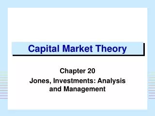
EFFICIENT FRONTIER FOR THE n-SECURITY CASE Expected return , E (Rp) • X • D F • Z• • B M • N • O • A Standard deviation,p
ASSUMPTIONS OF MARKOWITZ MODEL The Markowitz portfolio theory is based on a few assumptions i. Investors are risk-averse and thus have a preference for expected return and dislike for risk. ii. Investors act as if they make investment decisions on the basis of the expected return and the variance (or standard deviation) about security return distributions.
EVOLUTION OF CAPITAL ASSET PRICING MODEL (CAPM) • The CAPM was developed in the mid-1960s. The model has generally been attributed to William Sharpe, but John Lintner and Jan Mossin also made similar independent derivations. • Consequently, the model is often referred to as Sharpe-Lintner-Mossin (SLM) Capital Asset Pricing Model. • The CAPM explains the relationship that should exist between the securities’ expected returns and their risks in terms of the means and standard deviations.
ASSUMPTIONS OF CAPM • The capital market theory is built on the basis of Markowitz’s portfolio model. This theory is based on certain assumptions • All the investors are considered to be efficient investors who like to position themselves on the efficient frontier. • Investors are free to borrow or lend any amount of money at the Risk-Free Rate of Return (RFR). • All investors are expected to have homogeneous expectations. • All investors have same investment time horizons. • All investments are assumed to be infinitely divisible making it possible to even buy or sell fractional shares of any portfolio. • The process of buying or selling of assets does not involve any transaction costs. • It is assumed that the inflation rate is fully anticipated, or in other situation it may totally be absent thus resulting in no changes in the tax rate. • Another assumption of the theory is the equilibrium in the capital markets, that is, all the investments are correctly priced on par with their risk levels.
STANDARD DEVIATION Vs. BETA • Standard deviation is a measure of the dispersion of a set of data from its mean. The more spread apart the data, the higher the deviation. Standard deviation is calculated as the square root of variance. • Beta is a measure of the volatility, or systematic risk, of a security or a portfolio in comparison to the market as a whole. • one holding multiple assets, the contribution of any one of the assets to the riskiness of the portfolio is its systematic or non-diversifiable risk. Thus, for a well-diversified portfolio, the appropriate measure of risk would be beta.
RISK-FREE ASSETS In simple words, a risky asset is one which gives uncertain future returns whereas a risk-free asset whose expected return is fully certain and thus the standard deviation of such expected returns comes to zero, i.e., σf=0. Thus the rate of return earned on such assets should be the risk-free rate of return (rf).
COVARIANCE OF RISK-FREE ASSET WITH A RISKY ASSET The covariance between two sets of returns, A and B where asset A is a risk free asset. n CovAB = Σ[rA - E(rA)] [ rB - E(rB)]/n A=1 The uncertainty for a risk-free asset is known, so σA=0, which implies that rA = E(rA) for all the periods. Thus, rA - E(rA) =0, which further leads to the facts that the product of any other expressions with this expression will be zero. This will result in the covariance of the risk-free asset with any risky asset or portfolio to be also zero. Similarly, the correlation between any risky asset and risk-free asset, will be zero as rAB = CovA,B / σA σB.
COMBINING A RISK-FREE ASSET WITH A RISKY PORTFOLIO Any portfolio that combines a risk free asset with any risky asset, the standard deviation is the linear proportion of the standard deviation of the risky asset portfolio.
RISK-RETURN POSSIBILITIES WITH LEVERAGE An investor always wants to increase his expected returns. Say, a person has borrowed an amount which is 50 percent of his original wealth, the effect of this on the expected return for the portfolio would be: E(ri) = Wf (rf) + (1 - Wf) E(rk) where k is the risky assets portfolio = – 0.50 (rf) + [1 – (–0.50)] E(rk) = – 0.50 (rf) + 1.50 E(rk) Continued
Thus, we see that the return increases in a linear fashion along the line of risk-free rate (rf) and ‘k’. Now, suppose E(rf) = 0.10 And E(rk) = 0.24 E(ri) = = – 0.50 (0.10) + 1.5 (0.24) = 0.31 or 31% Similar is the effect of standard deviation of the leveraged portfolio. E(σi) = (1 – Wf) σk = [1 – (–0.5)] σk = 1.50 σk
D M C B A RFR Portfolio Possibilities Combining the Risk-Free Asset and Risky Portfolios on the Efficient Frontier
Risk Return Possibilities with Leverage in the diagram: • To attain a higher expected return than is available at point M (in exchange for accepting higher risk) • Either invest along the efficient frontier beyond point M, such as point D • Or, add leverage to the portfolio by borrowing money at the risk-free rate and investing in the risky portfolio at point M
Lending and Borrowing at the Riskfree rate The portfolio expected return for any portfolio i that combines f and M is E(ri) = WfRf + (1 – Wf) E (rM) Where, Wf = The percentage of the portfolio invested in the riskless security f 1 – Wf = The percentage of the portfolio invested in the risky portfolio M. The portfolio variance for portfolio i is: σi² =W²f σ²f + (1 - Wf)² σ²M + 2 Wf (1 - Wf) σf, M By definition, σ²f = 0. Thus, σ²i = (1 - Wf)² σ²M (or) σi = (1 - Wf) σM
CML Borrowing Lending M RFR Borrowing And Lending At Riskfee Rate Rf And Investing In The Risky Portfolio Dominant Portfolio “M”
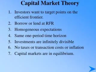
RISKLESS LENDING AND BORROWING OPPORTUNITY Expected return , E (Rp) G II V • E • X • • B S I • D • M • • F Y C • • • N u • • O Rf • • A Standard deviation,p Thus, with the opportunity of lending and borrowing, the efficient frontier changes. It is no longer AFX. Rather, it becomes Rf SG as it domniates AFX.
SEPARATION THEOREM • • Since Rf SG dominates AFX, every investor would do well to choose some combination of Rf and S. A conservative investor may choose a point like U, whereas an aggressive investor may choose a point like V. • • Thus, the task of portfolio selection can be separated into two steps: • Identification of S, the optimal portfolio of risky securities. • Choice of a combination of Rf and S, depending on one’s risk attitude. • This is the import of the celebrated separation theorem
Explanation : SEPARATION THEOREM • According to the portfolio theory, each investor should choose an appropriate portfolio along the efficient frontier. • The particular portfolio chosen may or may not involve borrowing or the use of leveraged, or short positions. The investment decision (to choose efficient portfolio from among others) and the financing decision (whether or not their portfolio involved borrowing, or short sales) are determined simultaneously in accordance with the risk level, identified by the investor at an acceptable level.
MARKET PORTFOLIO • A portfolio that contains all securities is called the Market Portfolio. Because all investors should choose the market portfolio, it should contain all available securities. • THE MARKET PORTFOLIO IN PRACTICE • It is a known fact that the market portfolio has all different kinds of stocks included, and when in equilibrium, the different assets included in the portfolio are in proportion to their market value. • Ideally, the market portfolio should not only contain stocks and bonds but also other assets such as coins, stamps, real estate and options, each assigned a different weight in proportion to their respective market values.
THE CAPITAL MARKET LINE (CML) • A line used in the capital asset pricing model to illustrate the rates of return for efficient portfolios depending on the risk-free rate of return and the level of risk (standard deviation) for a particular portfolio. • The CML is derived by drawing a tangent line from the intercept point on the efficient frontier to the point where the expected return equals the risk-free rate of return. • The CML is considered to be superior to the efficient frontier since it takes into account the inclusion of a risk-free asset in the portfolio • Thus the CML not only represents the new efficient frontier, but it also expresses the equilibrium pricing relationship between E(r) and σ for all efficient portfolios lying along the line.
CAPITAL MARKET LINE EXPECTED RETURN, E(Rp) Z • LM• • K RfSTANDARD DEVIATION, pE(Rj) = Rf + λ σj E(RM) - Rf λ = σM
THE CAPITAL ASSET PRICING MODEL (CAPM) A model that describes the relationship between risk and expected return and that is used in the pricing of risky securities. The general idea behind CAPM is that investors need to be compensated in two ways: time value of money and risk. The time value of money is represented by the risk-free (rf) rate in the formula and compensates the investors for placing money in any investment over a period of time. The other half of the formula represents risk and calculates the amount of compensation the investor needs for taking on additional risk. This is calculated by taking a risk measure (beta) that compares the returns of the asset to the market over a period of time and to the market premium (Rm-rf).
Explanation: • The CAPM states that the expected return of a security or a portfolio equals the rate on a risk-free security plus a risk premium. If this expected return does not meet or beat the required return, then the investment should not be undertaken. The security market line plots the results of the CAPM for all different risks (betas). • thus the CML is important in describing the equilibrium relationship between expected return and risk for efficient portfolios that contains no unsystematic risk. • Thus as per the CAPM model, the expected return of any asset is given by a formula of the form: • E[ri] = rf + [Number of Units of Risk][Risk Premium per Unit]
SECURITY MARKET LINE (SML) The SML essentially graphs the results from the capital asset pricing model (CAPM) formula. The x-axis represents the risk (beta), and the y-axis represents the expected return. The market risk premium is determined from the slope of the SML. E (R i ) = R f + [ E (R M)- R f ] β i
RELATIONSHIP BETWEEN SML AND CML SMLE(RM ) - RfE(Ri) = Rf + σiMσM 2SINCE σiM = iM σi σME(RM ) - RfE(Ri) = Rf + iM σi σM IF i AND M ARE PERFECTLY CORRELATED iM = 1. SOE(RM ) - RfE(Ri) = Rf + σi σM THUS CML IS A SPECIAL CASE OF SML
APPLICATION OF CML AND CAPM • There are a number of applications of ex post SML in security analysis and portfolio management. Among these are • Evaluating the performance of portfolios; • Tests of asset pricing theories; and • Tests of market efficiency Ex ante SML can be used to identify mispriced securities. It represents the liner relationship between the expected rates of return for securities and their expected betas.
PERFORMANCE EVALUATION OF PORTFOLIOS • The performance of portfolio is frequently evaluated based on the security market line criterion – • A large positive alpha being taken as an indicator of superior (above-normal) performance and • A large negative alpha being taken as an indicator of inferior (below-normal) performance.
TESTS OF ASSET PRICING THEORIES The CAPM pricing model is given by the equation: E(ri) = rf + [E(rM) – rf] βi According to the theory, the expected return on security i, E(ri), is related to the risk-free rate, rf, plus a risk premium, [E(rM) – rf] βi ,which includes the expected return on the market portfolio.
TESTS OF MARKET EFFICIENCY SML can also be used for testing market efficiency. As we know, when markets are efficient, the scope for abnormal return will not be there and returns on all securities will be commensurate with the underlying risk. That is, all assets are correctly priced and provide a normal return for their level of risk and the difference between return earned on the asset and required rate of return on the asset should be statistically insignificant if markets are efficient. IDENTIFYING MISPRICED SECURITIES The ex ante SML can be used for identifying mispriced (under and overvalued) securities.