Emissione delle Onde Sismiche
650 likes | 856 Vues
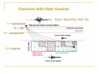
Emissione delle Onde Sismiche. R(f,x)= S(f,x) · P(f,x) · Ps(f) · I(f). I = registrazione. Ps = sito. P = propagazione. S = Sorgente. Il processo di rottura durante un terremoto. Spostamento (m). V r. Tempi di rottura (s). Accelerazioni del fronte di rottura (V r non è costante).

Emissione delle Onde Sismiche
E N D
Presentation Transcript
Emissione delle Onde Sismiche R(f,x)= S(f,x)·P(f,x) ·Ps(f) ·I(f) I = registrazione Ps = sito P = propagazione S = Sorgente
Il processo di rottura durante un terremoto Spostamento (m) Vr Tempi di rottura (s) Accelerazioni del fronte di rottura (Vr non è costante)
Parkfield Earthquakes:1934, 1966, 2004 slip from geodesy 1934 From Segall and Du * * 1966 From Segall and Du * 2004 From Jessica Murray
The 2002 M7.9 Denali, Alaska, earthquake • Where all that beautiful isochrone directivity stuff does not work because the rupture appears to travel faster than the S wave speed! • How does directivity work for supershear rupture speed?
Ground velocity at Pump Station 10, 2002 Denali earthquake Fault-normal Fault-parallel Vertical
Denali slip distribution Slip distribution of 2002 Denali, Alaska, earthquake From Eberhart-Phillips et al., Science, 2003 PS10 0 100 200 300 km
Slip (ss comp) and rupture time, model m14 PS10 3 km Subshear rupture velocity Supershear rupture velocity Slip, m Slip velocity function = decaying exponential, 1s time constant
PS10 data – m14 synthetic comparison observed (gray) synthetic (black) ground velocity. Note the one-sided FP pulse and the approximate simultaneity of the main peak on horizontal components. Critical data for supershear rupture.
Subshear and supershear isochrones isochrones and integrand for subshear rupture velocity isochrones and integrand for super-shear rupture velocity
PS10 affected by nearby portion of Denali Fault Fill colors show contribution of S wave radiation from each point to the fault-parallel displacement at PS10. Plot, for the portion of the Denali fault surface extending from the surface to 12 km depth and from 68 km east to 53 km west of PS10, located at 0 km along strike. Contours are isochrones of the arrival time function. Points within 5-10 km of PS10 at depths < 6 km dominate the motions at PS10. (from Ellsworth et al., Earthquake Spectra, 2004)
m14 isochrones, FP data and synthetics Lines – isochrones for supershear rupture model m14, colors – amplitude of S wave seen at PS10 Big pulse comes from infinite isochrone velocity at local minimum of arrival time function Black = synthetic, gray = observed 32.5
PS10 data – m14 synthetic comparison observed (gray) synthetic (black) ground velocity. What is this later energy??
Dunham and Archuleta PS10 model Snapshots of the fault surface with the color scale measuring slip velocity for model III (no healing, slip to 5km depth, shown every 1.65s). Time advances from bottom to top. The solid white lines show wave speeds (Rayleigh, S, and P from bottom to top). The dashed white line marks the position of the station.
Conclusions • A single station seismogram can be modeled many different ways (in other words, we could be wrong) • Supershear rupture velocity past PS10 explains the simultaneity of the FN and FP pulses, and the one-sided FP pulse • Pulse model – rise time was short (1/e time = 1 s) and peak slip velocity was 5 m/s • Perhaps later FN motion shows bifurcation of rupture front
EXPRIMENTAL METHODS 2) Ground-Motion Prediction Equations 1. Rock/Soil • Rock = less than 5m soil over granite, limestone, etc. • Soil = everything else 2. NEHRP Site Classes (Code prescribed amplification factors) 620 m/s = typical rock 310 m/s = typical soil
Theory Coefficienti di riflessione e rifrazione (onde SH) Superficie libera Materiale 2 r2, b2 At AMPIEZZE (incidenza verticale) • T12 = At / Ai = 2r1b1 / (r1b1+r2b2) = 2 / (1+a) • R12= Ar / Ai = (r1b1-r2b2) / (r1b1+r2b2) = (1-a)/(1+a) dove a = r2b2/r1b1contrasto d’impedenza • 1+ R12 = T12 (continuità dello spostamento) trasmessa interfaccia riflessa incidente Ar Ai Materiale 1 r1, b1
Theory Coefficienti di riflessione e rifrazione (onde SH) T12 = At / Ai = 2 / (1+a) R12= Ar / Ai = (1-a) / (1+a) incidenza verticaleincidenza obliqua a = r2b2 /r1b1 a = r2b2 cos j2 /r1b1cos j1 • Ovvero i coeff. di riflessione e trasmissione dipendono dall’angolo d’incidenza (e di emersione) • Per angolo d’incidenza < angolo critico, gran parte dell’energia viene trasmessa
Theory Coefficienti di riflessione e rifrazione (onde SH) T12 = 2 / (1+a) R12= (1-a)/(1+a) • Se α è < 1, l’onda incidente incontra un mezzo più “soffice”: l’onda trasmessa è maggiore della riflessa e l’onda riflessa ha lo stesso segno dell’onda incidente • Se α è > 1, l’onda incidente incontra un mezzo più “rigido”: l’onda trasmessa ha un’ampiezza minore e l’onda riflessa ha segno opposto dell’onda incidente • Se α =0,l’onda incontra una superficie libera (stress verticale non può essere trasmesso). Lo spostamento riflesso è uguale a quello incidente e si somma in fase (==spostamento trasmesso è due volte quello dell’onda incidente)
Theory Coefficienti di riflessione e rifrazione (onde SH) Esempi T12 = 2 / (1+a) R12= (1-a)/(1+a) • Se a=r2 b2 /r1 b1 = 0.2 T12 = 2.0 / 1.2 ~ 1.7 R12 = 0.8 / 1.2 ~ 0.7 • Se a=r2 b2 /r1 b1 = 0 T12= 2 superficie libera R12= 1 • Incidenza obliqua T12 e R12 dipendono dall’angolo d’incidenza (Per angolo d’incidenza < angolo critico, gran parte dell’energia viene trasmessa)
Theory Coefficienti di riflessione e rifrazione (onde SH) Esempio 1 Materiale 2 r2, b2 At • Se r2 b2 <<r1 b1 T12~ 2 R12 ~ 1 trasmessa Materiale 1 r1, b1 riflessa incidente Ai Ar ampiezza ampiezza onda trasmessa onda incidente!!! Com’è possibile??? ~ 2 x • Ė = E v = A2w2rv /2 flusso medio di energia attraverso l’unità di fronte d’onda si conserva
Theory Coefficienti di riflessione e rifrazione (onde SH) Esempio 2 At=2Ai • Se a=r2 b2 /r1 b1 = 0 T12=2 superficie libera R12=1 l’onda incidente Ai si somma in fase all’onda riflessa Ar dando luogo ad un’onda sulla superficie libera di ampiezza 2Ai Superficie libera Materiale 1 r1, b1 riflessa incidente Ai Ar
Theory MORE layers • Discontinuity in elastic properties causes multiple reflections of trapped waves, whose constructive interference causes resonance r2,Vs2 r1, Vs1 Vs1 > Vs2
Theory MORE layers: 1 layer overlying bedrock At=2 Ai At=-2 Ai Superficie libera Ar=Ai Materiale 2 Ai Ar=-Ai interfaccia incidente Materiale 1 (impedenza infinita)
Theory Tmp = At / Ai = 2 / (1+a) Rmp= Ar / Ai = (1-a) / (1+a) a=rpbp/rm bm 1 layer overlying bedrock Fase 1 At=2 Ai ro bo a= ro bo /r1 b1 =0 T1o =2 R1o= 1 r1 b1 Ai r2 b2 (∞)
Theory Tmp = At / Ai = 2 / (1+a) Rmp= Ar / Ai = (1-a) / (1+a) a=rpbp/rm bm 1 layer overlying bedrock Fase 1 At=2 Ai ro bo a= ro bo /r1 b1 =0 T1o =2 R1o= 1 r1 b1 Ai r2 b2 (∞) a= ro bo /r1 b1 =0 T1o =2 R1o= 1 Fase 2 At= - 2 Ai ro bo a= r2 b2 /r1 b1 =∞ T12 =0 R12= -1 Ar=Ai r1 b1 Ar=-Ai r2 b2 (∞)
Theory Tmp = At / Ai = 2 / (1+a) Rmp= Ar / Ai = (1-a) / (1+a) a=rpbp/rm bm 1 layer overlying bedrock Le onde rimangono “intrappolate” nell’interfaccia a= robo/r1 b1 =0 T1o =2 R1o= 1 ro bo At=2 Ai At=2 Ai At=-2 Ai Ar=Ai Ar=-Ai Ai r1 b1 Ar=Ai Ar=-Ai a= r2 b2 /r1 b1 =∞ T12 =0 R12= -1 r2 b2
Theory 1 layer overlying bedrock At=2 Ai At=-2 Ai At=2 Ai t1 to t2 t1-to=2h/v h to=h/v t2-to=4h/v Onda incidente
Theory 1 layer overlying bedrock At=2 Ai At=-2 Ai At=2 Ai t1 to t2 t1-to=2h/v h to=h/v t2-to=4h/v T=4h/v 2h/v to tempo
Theory 1 layer overlying bedrock T=4h/v tempo Se T=4h/v To, allora le onde riflesse si sovrappongono: RISONANZA To periodo onda incidente
Theory 1 layer overlying bedrock: Transfer Function Uniform layer of isotropic, linear elastic soil ovelying rigid bedrock (VERTICAL INCIDENCE) • The motion at bedrock produces propagating waves in the ovelying soil • Constructive interference of the upward and downward traveling waves produce STANDING waves • Standing wave has fixed shape with respect to H • (continue)
Theory 1 layer overlying bedrock: Transfer Function STANDING waves B r Vs H A z TRANSFER FUNCTION The Fourier amplitude of displacement in B (z=0) respect to A (z=H) will be: Amp_B(f) = F( f ) . Amp_A(f) where is the transfer function
Theory 1 layer overlying bedrock : Transfer Function • The amplitude is always >= 1 • The surface displacement reaches infinite amplification when F( f ) RESONANCE
Theory 1 layer overlying bedrock : Transfer Function • In generale, la funzione di trasferimento per uno strato omogeneo elastico su substrato rigido è periodica con periodo: armonica fondamentale armoniche superiori
Theory 1 layer overlying bedrock: Transfer Function • At each natural frequency, a standing wave develops in the soil waves F(f)
Theory Damping no inf inf 1 layer overlying bedrock + DAMPING The amplitude spectrum of a resonant system requires precise constructive interference of multiple arrivals. In practice this probably will not happen because of geologic complexity, and thus observations may not show a well-defined set of resonant peaks Realistic materials produce dissipation of energy (soil damping)
Theory B r1 V1 H A r2 V2 z 2 layers
Theory 2 layers
Theory B r1 V1 H A ∞ z B r1 V1 H A r2 V2 z 1 or 2 layers comparison • TRANSFER FUNCTION • For vertically incident SH-waves, the Fourier amplitude of displacement in B will be: Amp_B( f ) = F( f ) . Amp_A( f ) • 1 layer: • 2 layers: trasmission coef. reflection coef.
Theory 1 or 2 layers comparison • F( f ) Transfer function behavior • PEAKS occur when: • AMPLIFICATION occurs for f = fn: • 1 layer: F( fn ) = ∞ • 2 layers: (impedance ratio)
Theory Vs (m/sec) 0 100 200 300 400 500 0 2 layers 11:27:42 Time: 10 2004-01-05; Date: 20 (m) Depth B C:\site_amp\linear_gradient_steps_model.draw; 30 r1 V1 40 H A File: r2 V2 50 z 2 layers EXAMPLE (2 layers)
Theory 1 Z1 = 150*2 = 300 Z2 = 400*2 = 800 4 f = /4H = 150/(4*37.5) = 1 Hz 3 Z2/Z1 = 2.7 2 Response Site 1 2-step model 0.1 1 10 freq (Hz) 2 layers EXAMPLE (2 layers)
How do we estimate site effects? Numerical methods Output motion SITE Input motion
Esperimento Nocera Umbra Gli strati più superficiali sono in grado di amplificare le ampiezze delle onde sismiche ain funzione delle condizioni geologiche locali. Gli effetti di sito hanno un impatto enorme sulla distribuzione del movimento del terreno causato da un terremoto e del danno associato. Un esempio dal terremoto di Colfiorito Gli Effetti di Amplificazione dovuti alla geologia del Sito
Accelerometric model Source model after Capuano et al. (2000) and Zollo et al., 1999 Top of the fault: 3.4 km Max. depth : 8 km Uniform rupture velocity: 2.6 km/s Grid discretization: 10 m Slip distribution obtained by accelerometric data (Zollo et al., 1999 and Capuano et al., 2000)
Geodetic model 12 km Uniform rupture velocity: 0.9 Vs Source model after Hunstad et al., 2000 and Salvi et al., 2000 10 km Grid discretization: 10 m Slip distribution obtained by geodetic data ( Hunstad et al., 1999; Salvi et al., 2000)
Colfiorito training area - Task 2 • 1-D velocity model for the area (1st year): • We have used the genetic algorithm (GA) to obtain a set of best fitting 1-D P-wave seismic velocity structures (and mean VP / VS ratio) for the study area.