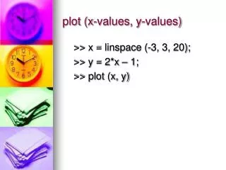
plot (x-values, y-values)
plot (x-values, y-values). >> x = linspace (-3, 3, 20); >> y = 2*x – 1; >> plot (x, y). xlabel (‘string’) ylabel (‘string’) title (‘string’). >> xlabel (‘x-axis’) >> ylabel (‘y-axis’) >> title (‘2D graph’). figure (n) hold on. >> t = linspace (0, 2*pi, 100);

plot (x-values, y-values)
E N D
Presentation Transcript
plot (x-values, y-values) >> x = linspace (-3, 3, 20); >> y = 2*x – 1; >> plot (x, y)
xlabel (‘string’)ylabel (‘string’)title (‘string’) >> xlabel (‘x-axis’) >> ylabel (‘y-axis’) >> title (‘2D graph’)
figure (n)hold on >> t = linspace (0, 2*pi, 100); >> y1 = sin(t); >> figure (2) >> plot (t, y1) >> y2 = cos(t) >> hold on >> plot (t, y2)
>>t = linspace (0, 2*pi, 100); >> y1 = sin(t); >> y2 = cos(t); >> plot (t, y1, ‘y’, t, y2, ‘r:-’) >> xlabel (‘t-axis’) >> ylabel (‘y-axis’) >> title (‘trigo curves’)
text (x-coordinate, y-coordinate, ‘string’) >> text (pi/2, 1, ‘y = sin t’) gtext (‘string’) >> gtext (‘y = cos t’) legend (‘string 1’, ‘string 2’, . . .) >> legend (‘y = sin t’, ‘y = cos t’)
axis ([xmin xmax ymin ymax]) >> y3 = tan(t); >> hold on >> plot (t, y3, ‘g : d’) >> axis ([0 7 -3 3])
line (xdata, ydata, property name, property value) >> y4 = sec(t); >> line (t, y4, ‘marker’, ‘+’)
area >> x = linspace (-3*pi, 3*pi, 100); >> y = -sin(x)./x; >> area (x, y)
comet >> q = linspace (0, 10*pi, 200); >> y = q.*sin(q); >> comet (q, y)
pie >> cont = char (‘Asia’, ‘Europe’, ‘Africa’, ‘N. America’, ‘S. America’); >> pop = [3332; 696; 694; 437; 307]; >> pie (pop) >> for I = 1 : 5, gtext (cont (i, :)); end
Stem >> t = linspace (0, 2*pi, 200); >> f = exp (-0.2*t).*sin(t); >> stem (t, f)
Stairs >> t = linspace (0, 2*pi, 200); >> r = sqrt (abs (2*sin(5*t))); >> y = r.*sin(t); >> stairs (t, y) >> axis ([0 pi 0 inf]);
Subplot (m, n, p)plot3 (x, y, z, ‘style-option’)xlabel (‘string’)ylabel (‘string’)zlabel (‘string’) >> t = linspace (0, 1, 100); >> x = t; y = t^; z = t ^ 3; >> subplot (2, 1, 1) >> plot3 (x, y, z, ‘r’)
grid >> grid view (a, b) >> subplot (2, 1, 2) >> view (60, 60) Comet3 >> t = linspace (0, 10*pi, 100); >> x = cos(t); >> y = sin(t); >> comet3 (t, x, y)