Bairstow's Method
340 likes | 696 Vues
Bairstow's Method is an iterative technique for finding roots of polynomials, blending concepts from both Müller’s and Newton-Raphson methods. This method employs a quadratic polynomial divisor and recursively calculates coefficients using a relation that facilitates adjustments to the parameters to minimize residual values. The steps involve inputting initial guesses, computing necessary coefficients, and iterating until convergence is achieved. This method is particularly effective for finding both real and complex roots simultaneously, making it a valuable tool in numerical analysis.

Bairstow's Method
E N D
Presentation Transcript
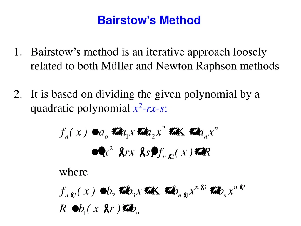
Bairstow'sMethod • Bairstow’s method is an iterative approach loosely related to both Müller and Newton Raphson methods • It is based on dividing the given polynomial by a quadratic polynomial x2-rx-s:
Bairstow'sMethod • 3. The coefficients b’s are obtained very easily by using recursive relation • 4. Using Newton Raphson approach, r and s are adjusted so as to make both bo and b1approach zero
Bairstow'sMethod • 5. Obtain corrections in r and s by Newton-Raphson method
Bairstow'sMethod • 6. Bairstow (1920) showed that the partial derivatives of b1 and b2 are obtained by the recursive relation • 7. Iterate the steps untill (Δr/r)and (Δs/s) drops below a specified threshold
Order of Convergence • Definition: Let be a sequence which converges to α. Define en = xn – α. If there exists a number p and a constant C ≠ 0 such that, Then, p is called the order of convergence of the sequence and C is the asymptotic error constant. • Fixed Point: = C, 1st Order. • Newton Raphson: = C, 2nd Order • Secant: = C, mixed order, ≈ 1.6 • Muller: = C, mixed order, ≈ 1.84
Polynomial Methods: Single Root If we divide by a factor (x - r) such that, r = α is a root of the polynomial, we will get an exact polynomial of order (n - 1), say . If r ≠ α, dividing by a factor (x - r) will have a remainder b0.
Polynomial Methods: Single Root For a given , are known. For a choice of r, one can determine from n+1 equations above having n+1 unknowns
Polynomial Methods: Single Root Remainder b0is a function of r → b0(r), at r = α, b0(r) = 0 Problem:f(x) = 0, find a root x = α such that f(α) = 0 Problem:b0(r) = 0, find a root r = α such that b0(α) = 0 Apply Newton-Raphson: Iteration Formula for Step k: or → b0’(r) = b1 → Assume a value of r, estimate b0 and b1, compute new r. Continue until b0 becomes zero. (with acceptable relative error)
Polynomial Methods: Bairstow's Let us divide by a factor (x2– rx – s). If the factor is exact, the resulting polynomial will be of order (n – 2). Two roots of the polynomial can be estimated simultaneously as the roots of the quadratic factor. For the complex roots, they will be the complex conjugates. If the factor (x2– rx – s) is not exact, there will be two remainder terms, one function of x and another constant. Let us express the remainder term as b1(x - r) + b0. This form instead of the standard b1x + b0 is chosen to device a convenient iteration formula!
Polynomial Methods: Bairstow's For a given , are known. For a choice of r and s, one can determine from n+1 equations above having n+1 unknowns
Polynomial Methods: Bairstow's b0 and b1 are functions of r and s → b0(r, s) and b1(r, s) Expand in Taylor’s series: Apply 2-d Newton-Raphson Need to evaluate: , , and
Polynomial Methods: Bairstow's Partial differentials with respect to r: = 0
Polynomial Methods: Bairstow's Partial differentials with respect to s: (say) = 0 = 0
Polynomial Methods: Bairstow's ; ; and For any given polynomial, we know {a0, a1, … an}. Assume r and s. Compute {b0, b1, … bn} and {c0, c1, … cn}. Compute Δr and Δs.
Polynomial Methods: Bairstow'sAlgorithm • Step 1: input a0, a1, … an and initialize r and s. • Step 2: compute b0, b1, … bn • Step 3: compute c0, c1, … cn • Step 4: compute Δr and Δs from • Step 5: compute rnew = r + Δr, snew = s + Δs • Step 6: check for convergence, and b0, b1 ≤ εʹ • Step 7: Stop if all convergence checks are satisfied. Else, set r = rnew, s = snew and go to step 2.
Bairstow'sMethod • Step 8. The roots quadratic polynomial x2-rx-sare obtained as • Step 9. At this point three possibilities exist: • The quotient is a third-order polynomial or greater. The previous values of r and s serve as initial guesses and Bairstow’s method is applied to the quotient to evaluate new r and s values. • The quotient is quadratic. The remaining two roots are evaluated directly, using the above eqn. • The quotient is a 1st order polynomial. The remaining single root can be evaluated simply as x=-s/r.
Example Problem Use initial guesses of r = s = -1 and iterate to εa ≤ 0.1% Soln: • Step 1:Input a0, a1, … an and initialize r and s. In Here n = 5; = 1.25; = -3.875; = 2.125; = 2.75; = -3.5; = 1;
Example Problem • Step 2: compute b0, b1, … bnusing recursive relations derived Here, n =5
Example Problem • Step 3: compute c0, c1, … cnusing recursive relations derived Here, n =5
Example Problem • Step 4: compute Δr and Δs from Here, Solving, = 0.3558 and = 1.1381 • Step 5: compute rnew = r + Δr, snew = s + Δs rnew = -1+ 0.3558 = -0.6442, snew= -1+ 1.1381 = 0.1381 • Step 6: check for convergence, ; b0, b1 ≤ εʹ =; =; • Step 7: Stop if all convergence checks are satisfied. Else, set r = rnew, s = snew and go to step 2.
Bairstow'sMethod • Step 8. The roots quadratic polynomial x2-rx-sare obtained as • Step 9. At this point three possibilities exist: • The quotient is a third-order polynomial or greater. The previous values of r and s serve as initial guesses and Bairstow’s method is applied to the quotient to evaluate new r and s values. • The quotient is quadratic. The remaining two roots are evaluated directly, using the above eqn. • The quotient is a 1st order polynomial. The remaining single root can be evaluated simply as x=-s/r.
Multiple Roots • Definition: A root α of the equation f(x) = 0 is said to have a multiplicity of q if, when, q > 1, the order of convergence is no longer valid. • Solution: Suppose a function f(x) is q-times continuously differentiable in the neighbourhood of a root α of multiplicity q, and where Define Therefore,α is a root of f(x) of multiplicity q but is a simple root of u(x)!
Revision of Solution of Non-linear Equations • Graphical Method – Provide insights but tedious/subjective • Bracketing methods • Bisection method • False position method • Modified false position method • Open methods • Fixed-point iteration • Newton-Raphson • Secant & Modified Secant Guaranteed convergence Linear or better convergence May diverge FP - linear convergence NR – quadratic convergence Secant – between linear & quadratic NR – problems near zero gradient
Revision of Solution of Non-linear Equations • Hybrid Methods • Dekker method • Brent method • Multiple roots • Bracketing method – Only for odd number of roots • Newton-Raphson - Linear convergence • Modified Newton Raphson – Quadratic convergence • Known multiplicity • Derivative function • Combination • Bracketing method at the beginning • Open method near convergence
Revision of Solution of Non-linear Equations • Roots of polynomials • Evaluation of polynomials • Division of polynomials • Deflation of polynomials • Effective degree of polynomials • Method of finding roots • Müller method • Bairstow'smethod Real and complex rooots
Revision of Solution of Non-linear Equations Except for rare cases, computers will provide approximate solution. No method is “universally” better than others. Domain knowledge should guide the selection of algorithm and guess value(s).