Understanding Network Layer Services: Routing, Path Selection, and IPv6 Implementation
This chapter explores the essential principles of network layer services, focusing on routing and path selection. It delves into hierarchical routing, the Internet Protocol (IP), and the inner workings of routers. Additionally, it addresses advanced topics, including the implementation of IPv6 and mobility within the Internet architecture. Key concepts are covered, such as intra-domain and inter-domain routing protocols, the functions of routers, the differences between virtual circuits and datagram services, and the evolution of network technologies to accommodate new services in a diverse application landscape.

Understanding Network Layer Services: Routing, Path Selection, and IPv6 Implementation
E N D
Presentation Transcript
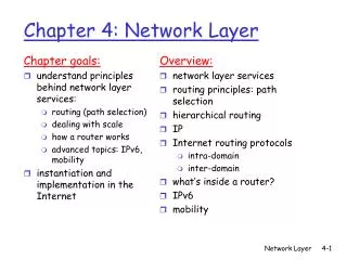
Chapter goals: understand principles behind network layer services: routing (path selection) dealing with scale how a router works advanced topics: IPv6, mobility instantiation and implementation in the Internet Overview: network layer services routing principles: path selection hierarchical routing IP Internet routing protocols intra-domain inter-domain what’s inside a router? IPv6 mobility Chapter 4: Network Layer Network Layer
Chapter 4 roadmap 4.1 Introduction and Network Service Models 4.2 Routing Principles 4.3 Hierarchical Routing 4.4 The Internet (IP) Protocol 4.5 Routing in the Internet 4.6 What’s Inside a Router 4.7 IPv6 4.8 Multicast Routing Network Layer
transport packet from sending to receiving hosts network layer protocols in every host, router three important functions: path determination: route taken by packets from source to dest. Routing algorithms forwarding: move packets from router’s input to appropriate router output call setup: some network architectures require router call setup along path before data flows network data link physical network data link physical network data link physical network data link physical network data link physical network data link physical network data link physical network data link physical application transport network data link physical application transport network data link physical Network layer functions Network Layer
Q: What service model for “channel” transporting packets from sender to receiver? guaranteed bandwidth? preservation of inter-packet timing (no jitter)? loss-free delivery? in-order delivery? congestion feedback to sender? Network service model The most important abstraction provided by network layer: ? ? virtual circuit or datagram? ? service abstraction Network Layer
call setup, teardown for each call before data can flow each packet carries VC identifier (not destination host ID) every router on source-dest path maintains “state” for each passing connection transport-layer connection only involved two end systems link, router resources (bandwidth, buffers) may be allocated to VC to get circuit-like perf. “source-to-dest path behaves much like telephone circuit” performance-wise network actions along source-to-dest path Virtual circuits Network Layer
used to setup, maintain teardown VC used in ATM, frame-relay, X.25 not used in today’s Internet application transport network data link physical application transport network data link physical Virtual circuits: signaling protocols 6. Receive data 5. Data flow begins 4. Call connected 3. Accept call 1. Initiate call 2. incoming call Network Layer
no call setup at network layer routers: no state about end-to-end connections no network-level concept of “connection” packets forwarded using destination host address packets between same source-dest pair may take different paths application transport network data link physical application transport network data link physical Datagram networks: the Internet model 1. Send data 2. Receive data Network Layer
Evolution of ATM-Based B-ISDN ATM – Asynchronous Transfer Mode B-ISDN – Broadband Integrated Services Digital Networks • ISDN failed because • It had low transmission rates to be able to support the new emerging applications • Did not support integration of services over the same channel (at the physical/link levels) • New technology has emerged • Optical networks – low error rates • High-speed switching Network Layer
New services and Traffic • A number of new services needed to be supported – Video, voice, data, streaming • These have different traffic characteristics • Peak rate (PCR) • Mean (sustainable) Rate (SCR) • Minimum Rate (MCR) • Burst Size (MBS) • and different Quality of Service Requirements • End-to-end delay (CTD) • Delay jitter (SDV) • Error rate (CER) • Routing accuracy (CMR) Network Layer
Evolution of B-ISDN (cont.) • Traditional networks have been designed and optimized for a single application (e.g., voice, video, data, telegraph) • A large number of services have emerged, e.g., HDTV, video conferencing, medical imaging, distant learning, video on demand, electronic commerce, etc. • It is more economical and cost effective to serve all these applications by one network • This trend is facilitated by the evolution in the semiconductor, optical technologies, and the shifting transport functions to network periphery, which reduced cost of services Network Layer
Evolution of B-ISDN (cont.) • The (narrowband) Integrated Services Digital Network (ISDN) was one step in this direction: integrated voice & data services • Problems: • - limited maximum bandwidth (2 Mbits/sec max) • - based on circuit switching (64 Kbits/sec) advances in data compression are not directly supported by (N)ISDN switches Network Layer
Range of Services for B-ISDN Network Layer
Transfer Modes • A transfer mode is a technique which is used in a telecommunication network covering aspects related to transmission, multiplexing and switching • A transfer mode should provide flexibility & adaptability to varying bit rates Since B-ISDN required flexibility, but at the same time must employ network wide lightweight protocols,modes near the middle of the spectrum were a good compromise – Hence ATM. Network Layer
Operational Characteristics • No error protection inside the network (handled by higher layers) • No flow control on a link-by-link basis • Connection-oriented mode: • Quality of Service (QOS) guarantees • Lightweight routing decisions • Reduced header functionality (mainly routing): fast processing & high throughputs • The information field is relatively small: • high degree of pipelining (emulation of cut-through) • small delay & delay jitter Network Layer
ATM Service Categories • Real time • Constant bit rate (CBR) • Real time variable bit rate (rt-VBR) • Non-real time • Non-real time variable bit rate (nrt-VBR) • Available bit rate (ABR) • Unspecified bit rate (UBR) Network Layer
Real Time Services • Amount of delay • Variation of delay (jitter) Network Layer
CBR • Fixed data rate continuously available • Tight upper bound on delay • Uncompressed audio and video • Video conferencing • Interactive audio • A/V distribution and retrieval Network Layer
rt-VBR • Time sensitive application • Tightly constrained delay and delay variation • rt-VBR applications transmit at a rate that varies with time • e.g. compressed video • Produces varying sized image frames • Original (uncompressed) frame rate constant • So compressed data rate varies • Can statistically multiplex connections Network Layer
nrt-VBR • May be able to characterize expected traffic flow • Improve QoS in loss and delay • End system specifies: • Peak cell rate • Sustainable or average rate • Measure of how bursty traffic is • e.g. Airline reservations, banking transactions Network Layer
UBR • May be additional capacity over and above that used by CBR and VBR traffic • Not all resources dedicated • Bursty nature of VBR • For application that can tolerate some cell loss or variable delays • e.g. TCP based traffic • Cells forwarded on FIFO basis • Best effort service Network Layer
ABR • Application specifies peak cell rate (PCR) and minimum cell rate (MCR) • Resources allocated to give at least MCR • Spare capacity shared among all ABR sources • e.g. LAN interconnection Network Layer
ATM Bit Rate Services Network Layer
Network layer service models: Guarantees ? Network Architecture Internet ATM ATM ATM ATM Service Model best effort CBR VBR ABR UBR Congestion feedback no (inferred via loss) no congestion no congestion yes no Bandwidth none constant rate guaranteed rate guaranteed minimum none Loss no yes yes no no Order no yes yes yes yes Timing no yes yes no no • Internet model being extended: Intserv, Diffserv • Chapter 6 Network Layer
Internet data exchange among computers “elastic” service, no strict timing req. “smart” end systems (computers) can adapt, perform control, error recovery simple inside network, complexity at “edge” many link types different characteristics uniform service difficult ATM evolved from telephony human conversation: strict timing, reliability requirements need for guaranteed service “dumb” end systems telephones complexity inside network Datagram or VC network: why? Network Layer
Chapter 4 roadmap 4.1 Introduction and Network Service Models 4.2 Routing Principles • Link state routing • Distance vector routing 4.3 Hierarchical Routing 4.4 The Internet (IP) Protocol 4.5 Routing in the Internet 4.6 What’s Inside a Router 4.7 IPv6 4.8 Multicast Routing Network Layer
Graph abstraction for routing algorithms: graph nodes are routers graph edges are physical links link cost: delay, $ cost, or congestion level A D B E F C Routing protocol Routing 5 Goal: determine “good” path (sequence of routers) thru network from source to dest. 3 5 2 2 1 3 1 2 1 • “good” path: • typically means minimum cost path • other def’s possible Network Layer
Global or decentralized information? Global: all routers have complete topology, link cost info “link state” algorithms Decentralized: router knows physically-connected neighbors, link costs to neighbors iterative process of computation, exchange of info with neighbors “distance vector” algorithms Static or dynamic? Static: routes change slowly over time Dynamic: routes change more quickly periodic update in response to link cost changes Routing Algorithm classification Network Layer
Dijkstra’s algorithm net topology, link costs known to all nodes accomplished via “link state broadcast” all nodes have same info computes least cost paths from one node (‘source”) to all other nodes gives routing table for that node iterative: after k iterations, know least cost path to k dest.’s Notation: c(i,j): link cost from node i to j. cost infinite if not direct neighbors D(v): current value of cost of path from source to dest. V p(v): predecessor node along path from source to v, that is next v N: set of nodes whose least cost path definitively known A Link-State Routing Algorithm Network Layer
Dijsktra’s Algorithm 1 Initialization: 2 N = {A} 3 for all nodes v 4 if v adjacent to A 5 then D(v) = c(A,v) 6 else D(v) = infinity 7 8 Loop 9 find w not in N such that D(w) is a minimum 10 add w to N 11 update D(v) for all v adjacent to w and not in N: 12 D(v) = min( D(v), D(w) + c(w,v) ) 13 /* new cost to v is either old cost to v or known 14 shortest path cost to w plus cost from w to v */ 15 until all nodes in N Network Layer
A D E B F C Dijkstra’s algorithm: example D(B),p(B) 2,A 2,A 2,A D(D),p(D) 1,A D(C),p(C) 5,A 4,D 3,E 3,E D(E),p(E) infinity 2,D Step 0 1 2 3 4 5 start N A AD ADE ADEB ADEBC ADEBCF D(F),p(F) infinity infinity 4,E 4,E 4,E 5 3 5 2 2 1 3 1 2 1 Network Layer
Algorithm complexity: n nodes each iteration: need to check all nodes, w, not in N n*(n+1)/2 comparisons: O(n**2) more efficient implementations possible: O(nlogn) Oscillations possible: e.g., link cost = amount of carried traffic A A A A D D D D B B B B C C C C Dijkstra’s algorithm, discussion 1 1+e 2+e 0 2+e 0 2+e 0 0 0 1 1+e 0 0 1 1+e e 0 0 0 e 1 1+e 0 1 1 e … recompute … recompute routing … recompute initially Network Layer
iterative: continues until no nodes exchange info. self-terminating: no “signal” to stop asynchronous: nodes need not exchange info/iterate in lock step! distributed: each node communicates only with directly-attached neighbors Distance Table data structure each node has its own row for each possible destination column for each directly-attached neighbor to node example: in node X, for dest. Y via neighbor Z: distance from X to Y, via Z as next hop X = D (Y,Z) Z c(X,Z) + min {D (Y,w)} = w Distance Vector Routing Algorithm Network Layer
cost to destination via E D () A B C D A 1 7 6 4 B 14 8 9 11 D 5 5 4 2 destination A D B E C E E E D (C,D) D (A,D) D (A,B) D D B c(E,D) + min {D (C,w)} c(E,D) + min {D (A,w)} c(E,B) + min {D (A,w)} = = = w w w = = = 8+6 = 14 2+2 = 4 2+3 = 5 Distance Table: example 1 7 2 8 1 2 loop! loop! Network Layer
cost to destination via E D () A B C D A 1 7 6 4 B 14 8 9 11 D 5 5 4 2 destination Distance table gives routing table Outgoing link to use, cost A B C D A,1 D,5 D,4 D,4 destination Routing table Distance table Network Layer
Iterative, asynchronous: each local iteration caused by: local link cost change message from neighbor: its least cost path change from neighbor Distributed: each node notifies neighbors only when its least cost path to any destination changes neighbors then notify their neighbors if necessary wait for (change in local link cost of msg from neighbor) recompute distance table if least cost path to any dest has changed, notify neighbors Distance Vector Routing: overview Each node: Network Layer
Distance Vector Algorithm: At all nodes, X: 1 Initialization: 2 for all adjacent nodes v: 3 D (*,v) = infinity /* the * operator means "for all rows" */ 4 D (v,v) = c(X,v) 5 for all destinations, y 6 send min D (y,w) to each neighbor /* w over all X's neighbors */ X X X w Network Layer
Distance Vector Algorithm (cont.): 8 loop 9 wait (until I see a link cost change to neighbor V 10 or until I receive update from neighbor V) 11 12 if (c(X,V) changes by d) 13 /* change cost to all dest's via neighbor v by d */ 14 /* note: d could be positive or negative */ 15 for all destinations y: D (y,V) = D (y,V) + d 16 17 else if (update received from V wrt destination Y) 18 /* shortest path from V to some Y has changed */ 19 /* V has sent a new value for its min DV(Y,w) */ 20 /* call this received new value is "newval" */ 21 for the single destination y: D (Y,V) = c(X,V) + newval 22 23 if we have a new min D (Y,w)for any destination Y 24 send new value of min D (Y,w) to all neighbors 25 26 forever X X w X X w X w Network Layer
2 1 7 X Z Y Distance Vector Algorithm: example Network Layer
2 1 7 Y Z X X c(X,Y) + min {D (Z,w)} c(X,Z) + min {D (Y,w)} D (Y,Z) D (Z,Y) = = w w = = 2+1 = 3 7+1 = 8 X Z Y Distance Vector Algorithm: example Network Layer
X Z Y Distance Vector: link cost changes Link cost changes: • node detects local link cost change • updates distance table (line 15) • if cost change in least cost path, notify neighbors (lines 23,24) 1 4 1 50 algorithm terminates “good news travels fast” Network Layer
X Z Y Distance Vector: link cost changes Link cost changes: • good news travels fast • bad news travels slow - “count to infinity” problem! 60 4 1 50 algorithm continues on! Network Layer
X Z Y Distance Vector: poisoned reverse If Z routes through Y to get to X : • Z tells Y its (Z’s) distance to X is infinite (so Y won’t route to X via Z) • will this completely solve count to infinity problem? 60 4 1 50 algorithm terminates Network Layer
Example • Consider the following network. Let the delay distance vector at nodes A, I, H and K be as given below, and let their respective measured distance to node J be 6, 9, 13 and 5. What will the routing table at node J look like after the next information exchange? Put the answer in the box below. Network Layer
Message complexity LS: with n nodes, E links, O(nE) msgs sent each DV: exchange between neighbors only convergence time varies Speed of Convergence LS: O(n2) algorithm requires O(nE) msgs may have oscillations DV: convergence time varies may be routing loops count-to-infinity problem Robustness: what happens if router malfunctions? LS: node can advertise incorrect link cost each node computes only its own table DV: DV node can advertise incorrect path cost each node’s table used by others error propagate thru network Comparison of LS and DV algorithms Network Layer
Chapter 4 roadmap 4.1 Introduction and Network Service Models 4.2 Routing Principles 4.3 Hierarchical Routing 4.4 The Internet (IP) Protocol • 4.4.1 IPv4 addressing • 4.4.2 Moving a datagram from source to destination • 4.4.3 Datagram format • 4.4.4 IP fragmentation • 4.4.5 ICMP: Internet Control Message Protocol • 4.4.6 DHCP: Dynamic Host Configuration Protocol • 4.4.7 NAT: Network Address Translation 4.5 Routing in the Internet 4.6 What’s Inside a Router 4.7 IPv6 4.8 Multicast Routing Network Layer
Host, router network layer functions: • ICMP protocol • error reporting • router “signaling” • IP protocol • addressing conventions • datagram format • packet handling conventions • Routing protocols • path selection • RIP, OSPF, BGP forwarding table The Internet Network layer Transport layer: TCP, UDP Network layer Link layer physical layer Network Layer
IP address: 32-bit identifier for host, router interface interface: connection between host/router and physical link router’s typically have multiple interfaces host may have multiple interfaces IP addresses associated with each interface 223.1.1.2 223.1.2.2 223.1.2.1 223.1.3.2 223.1.3.1 223.1.3.27 IP Addressing: introduction 223.1.1.1 223.1.2.9 223.1.1.4 223.1.1.3 223.1.1.1 = 11011111 00000001 00000001 00000001 223 1 1 1 Network Layer
IP address: network part (high order bits) host part (low order bits) What’s a network ? (from IP address perspective) device interfaces with same network part of IP address can physically reach each other without intervening router IP Addressing 223.1.1.1 223.1.2.1 223.1.1.2 223.1.2.9 223.1.1.4 223.1.2.2 223.1.1.3 223.1.3.27 LAN 223.1.3.2 223.1.3.1 network consisting of 3 IP networks (for IP addresses starting with 223, first 24 bits are network address) Network Layer
How to find the networks? Detach each interface from router, host create “islands of isolated networks IP Addressing 223.1.1.2 223.1.1.1 223.1.1.4 223.1.1.3 223.1.7.0 223.1.9.2 223.1.9.1 223.1.7.1 223.1.8.1 223.1.8.0 223.1.2.6 223.1.3.27 Interconnected system consisting of six networks 223.1.2.1 223.1.2.2 223.1.3.1 223.1.3.2 Network Layer
multicast address 1110 network host 110 network 10 host IP Addresses given notion of “network”, let’s re-examine IP addresses: “class-full” addressing: class 1.0.0.0 to 127.255.255.255 A network 0 host 128.0.0.0 to 191.255.255.255 B 192.0.0.0 to 223.255.255.255 C 224.0.0.0 to 239.255.255.255 D 32 bits Network Layer