Real-Time Optimization (RTO) In previous chapters we have emphasized control
390 likes | 414 Vues
Learn how Real-Time Optimization (RTO) enhances control system performance by optimizing set points for efficient operation. Explore key processes, problems, and solutions in chemical plant optimization.

Real-Time Optimization (RTO) In previous chapters we have emphasized control
E N D
Presentation Transcript
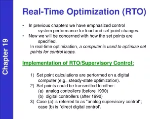
Real-Time Optimization (RTO) • In previous chapters we have emphasized control • system performance for load and set-point changes. • Now we will be concerned with how the set points are • specified. • In real-time optimization, a computer is used to optimize set points for control loops. • Implementation of RTO/Supervisory Control: • 1) Set point calculations are performed on a digital • computer (e.g., steady-state optimization). • 2) Set points could be transmitted to either: • (a) analog controllers (before 1990) • (b) digital controllers (after 1990) • 3) Case (a) is referred to as "analog supervisory control"; • case (b) is "direct digital control'. Chapter 19
Selection of Processes for RTO • Sources of information for the analysis: • 1) Profit and loss statements for the plant • Sales, prices • Manufacturing costs etc. • 2) Operating records • Material and energy balances • Unit efficiencies, production rate etc. • Categories of Interest: • 1) Sales limited by production • Increases in throughput desirable • Incentives for improved operating conditions and schedules. • 2) Sales limited by market • Seek improvements in efficiency. • Example: Reduction in manufacturing costs (utilities, feedstocks) • 3) Large throughput units • Small savings in production costs per unit are greatly magnified. Chapter 19
4) Process Variability • Excursions in process variables => offspec products and a need for larger storage capacities. • Reduction in variability allows set points to be moved closer to a limiting constraint, e.g. product quality. Chapter 19
5) High Raw Material or Energy Consumption • e.g., Minimize energy consumption by optimal allocation of fuel supplies and steam. • 6) Losses of Valuable Components in waste Streams • Detect via chemical analysis plant exit streams (e.g., air and water). Adjust air/fuel ratio in furnace to minimize hydrocarbon consumption. Chapter 19
Common Types of Optimization Problems • 1. Operating Conditions • Tower reflux ratio • Reactor temperature • 2. Allocation • Fuel use • Feedstock selection • 3. Scheduling • Cleaning (e.g., heat exchangers) • Maintenance • Batch processes Chapter 19
Formulation and Solution of Optimization Problems (see book by Edgar et al., “Optimization of Chemical Processes”) • In order to perform on-line optimization, a series of steps are required: • Step 1: Determine the process variables of interest. • Step 2: Definition of the Objective Function • Difficult part of the problem! • Example: Minimize the amount of offspec product from a • distillation column while avoiding a flooding condition. • - Relate off-spec product to costs of utilities and feedstocks. • Treat flooding condition as a constraint on vapor and • liquid flow rates. • Specific objective functions will depend on plant configuration • and supply and demand. Chapter 19 (See TABLE 1 - next slide)
Step 3. Development of Process Models • Process model is used in on-line optimization. Consists of: • - Equality constraints which relate principal process variables. • - Inequality constraints (e.g., physical limits on pumps, compressors, metallurgical limits) • Process model is usually a steady-state model. • Some batch optimization methods use the process as the model. (e.g., design of experiments) Chapter 19
Step 4. Simplification of the Process Model • Reduce the size of the optimization problem as much as • possible without losing the essence of the problem. • - Ignore process variables which have a negligible effect on • the objective function. • Step 5. Computation of the Optimum • Choose a computational technique to determine optimum. • Virtually all optimization techniques are iterative in nature – • linear programming, nonlinear programming. • Good estimate of the optimum accelerates convergence. • - Experience on which inequality constraints might be active is • also useful. • Step 6. Sensitivity Studies • Can be used to determine which variables and parameters • are most important in determining the optimum. Chapter 19
One Dimensional Search Techniques • Selection of a method involves a trade-off between the number of objective function evaluations (computer time) and complexity. • (1) "Brute Force" Approach • Small grid spacing (x) and evaluate f(x) at each grid point can get close to the optimum but very inefficient. • (2) Equal Interval Search • Example: Compare objective function values at 3 equally spaced points. • Suppose we are interested in the region, a x b . Thus initially, the "region of uncertainty, L" is L0 = b - a . • Consider two cases: Chapter 19
Chapter 19 • For case (1), maximum lies in (x2, b) • For case (2), maximum lies in (x1, x3)
Polynomial fitting technique • Fit quadratic polynomial to three data points. Find analytical optimum, then calculate f(x*). Discard worst value of f, then repeat the process. Chapter 19
Multivariable Optimization • Computational efficiency is important. • "Brute force" techniques are not practical for problems with • more than 3 or 4 variables to be optimized. • Typical Approach: Reduce the multivariable optimization • problem to a series of one dimensional problems: • (1) From a given starting point, specify a search direction. • (2) Find the optimum along the search direction, i.e., a • one-dimensional search. • (3) Determine a new search direction. • (4) Repeat steps (2) and (3) until the optimum is located • Two general categories for MV optimization techniques: • (1) Methods requiring derivatives of the objective function. • (2) Methods that do not require derivatives. Chapter 19
Nonderivative methods are attractive for real-time optimization • applications where a process measurement is used in place • of the objective function. • Two nonderivative methods which have been used in industrial • applications: • (1) Evolutionary Operation (EVOP) • (2) Simplex or Pattern Search Method. • Evolutionary Operation (EVOP) • Procedure: • (1) Choose a base point. • (2) Evaluate objective function at base point and a set of • regularly spaced points around the base point. • For 2 variables, form a square around the base point. • For 3 variables, form a cube. • (3) Move the process to the point that has the largest value • of the objective function. • (4) Use this point as the new base point. • (5) Repeat steps (2) and (4) until no further improvement • occurs. Chapter 19
Disadvantage of EVOP: • - It is slow due to the large number of steadystate points • which must be evaluated at each iteration. • Sequential Simplex Method [8] • Uses a regular geometric figure (a simplex) as a basis. • - Two variable problem: use an equilateral triangle. • - Three variable problem: use a regular tetrahedron. • Objective function is evaluated at the vertices of the simplex. • General direction of search is projected away form the worst • vertex. • Thus search direction can change and only one new operating • point must be evaluated at each iteration. • Example: The two variable problem, max f(x1, x2) Chapter 19 Assume
Points 2,3, and 4 form a new equilateral triangle. • The pattern search approach usually results in a zig-zag • pattern as it moves to the optimum (see figure 20.6- • next slide). • Constrained Optimization • Optimization problems commonly involve equality and • inequality constraints. • Nonlinear Programming (NLP) Problems: • a) Involve nonlinear objective function (and possible • nonlinear constraints). • b) Efficient off-line optimization methods are available (e.g. • conjugate gradient, variable metric). • c) On-line use? May be limited by computer time and • storage requirements. • Quadratic Programming (QP) Problems: • a) Quadratic objective function plus linear equality and • inequality constraints. • b) Computationally efficient methods are available. Chapter 19
Linear Programming (LP) Problems • Both objective function and constraints are linear. • Solutions are highly structured and can be rapidly obtained. • Linear Programming (LP) • Has gained widespread industrial acceptance for on-line • optimization, blending etc. • Linear constraints can arise due to: • 1. Production limitation e.g. equipment limitations, storage • limits, market constraints. • 2. Raw material limitation • 3. Safety restrictions, e.g. allowable operating ranges for • temperature and pressures. • 4. Physical property specifications e.g. product quality • constraints when a blend property can be calculated as • an average of pure component properties: Chapter 19
5. Material and Energy Balances • - Tend to yield equality constraints. • - Constraints can change frequently, e.g. daily or hourly. • Effect of Inequality Constraints • - Consider the linear and quadratic objective functions on • the next page. • - Note that for the LP problem, the optimum must lie on one • or more constraints. • General Statement of the LP Problem: • subject to: • Solution of LP Problems • - Simplex Method • - Examine only constraint boundaries • - Very efficient, even for large problems Chapter 19
Chapter 19 The effect of an inequality constraint on the maximum of quadratic function, (The arrows indicate the allowable values of x.)
Most LP applications involve more than two variables • and can involve 1000s of variables. • So we need a more general computational approach, • based on the Simplex method. There are many • variations of the Simplex method. • One that is readily available is the Excel Solver. • Basic features of LP: • Linear objective function • Linear equality/inequality constraints Chapter 19
Nonlinear Programming (NLP) example -nonlinear objective function -nonlinear constraints Chapter 19
Chapter 19 Previous chapter Next chapter
