Stochastic Parameter Optimization for Empirical Molecular Potentials
This work explores the application of stochastic parameter optimization methods, particularly simulated annealing, to derive empirical molecular potentials and tightly bound parameters. By optimizing the function that simulates the dynamics of atomic structures, we aim to calculate total energy and forces acting on atoms within large molecular systems. The goal is to achieve a local minimum on the Potential Energy Surface (PES) while fitting parameters to experimental results. While the method shows promise, challenges include potential entrapment in local minima and the necessity of representative sampling in high-dimensional spaces.

Stochastic Parameter Optimization for Empirical Molecular Potentials
E N D
Presentation Transcript
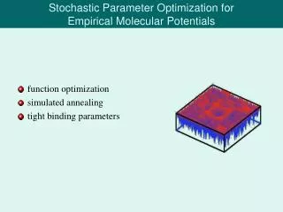
Stochastic Parameter Optimization for Empirical Molecular Potentials • function optimization • simulated annealing • tight binding parameters
Motivation • simulate dynamics of atomic structures • derive total energy and forces acting on atoms • empirical potentials + fit parameters to experiment soft spheres: only distance dependent • quantum mechanics: electrons dominate bonding • millions of atoms: approximate electronic degree of freedom • semi-empirical: capture QM origin of bonding tight binding: provides directional bonding • fit simulated properties to experimental ones • more approximations: more parameters to adjust • BOP4 potential : 11 parameters [material/compound] automatic fit procedure providing one or more good parameter sets
Optimization • find optimal solution to given problem such as: • economy: shortest itinerary between number of cities (traveling salesman) • engineering: drug design/ circuit design • quantify the problem • ‘goodness’ of solution depends on parameters objective function • set of parameters state in vector space • goal: find best local minimum on Potential Energy Surface (PES) • cost function :recover exp. properties, some better than others find point in 11-D continous space
Deterministic Methods (downhill only) • 1D Golden Section Search • higher dimensions: • Steepest Descent • Conjugate Gradient • Variable Metric • downhill simplex (no derivative)
Monte Carlo • statistical physics: access ensemble averages • magnetization of Ising model • higher energy states less probable • trick: don’t weigh all possible states , but only representative subset • simple sampling: waste time on states, that don’t contribute • importance sampling: arithmetic mean ?how to judge importance without prior knowledge of energy reference?
Metropolis Algorithm • judge upon relative energy-difference to previous state • guarantee detailed balance of hopping between states • Metropolis-function: transition probability • Metropolis et al. (1953) : find optimal wiring (min. length) on chip • allow for uphill climbing: move to neighboring local minima
Simulated Annealing propose new state accept reject update TopList lower T in intervals • in analogy to anneal process of metals: • slower cooling: better crystalization (energetically lower state) • faster cooling: freezing small crystals (higher, local minimum) • Kirkpatrick et al. (1983) added T-schedule to Metropolis search • search parameter space at successively lower temperature (higher ) : • T controls: • scale on which parameters are randomly changed: • prob. at which costly uphill moves are accepted: • find global minimum on PES for logarithmic annealing (single crystal) • in practice: simulated quenching with exponential cooling scheme
Traveling Salesman • visit all cities: combinatorial problem • minimize salesman’s way • different cost for crossing the river: minimize salesman’s cost equal weight: smuggler: river penalty:
Variations of the Theme: Statistic Tunneling (ST) • simulated quenching is prone to freezing • process is trapped in a deep local (but not global) minimum, that is surrounded by higher intermediate states -or- • very good (perhaps global) minimum is surrounded by higher states (on mountain top) and might never be found • transform PES: • ‘tunnel’ through forbidden, higher regions • preserve/amplify lower lying regions • effectively raising T in higher regions
Tight Binding (TB) Parameters • molecular wavefunction is linear combination of atomic wf. • replace hopping integral with parameter • angular dependence was given by Slater and Koster (1954) and is fitted to band structures of periodic systems • dynamic modeling needs continuous distance dependence • heuristic shape guided by radial solutions such as: • choice of dist. dep. is the integral part of TB • total energy:
Radial Dependence • repulsive potential and bond integral scale with same functional form • separate scaling parameter for -bonds and repulsive potential following • common cut-off parameter • #of parameters for s-p-bonded system: 3x2(scaling)+1(cutoff)+ 3(screening)+1(promotion)=11 • strong repulsion at and strong attraction at equilibrium at
Fitting BOP4 • cost-function: equilibrium values of • bulk modulus • rem. elastic constants • lattice parameter • cohesive energy • lattice parameter for graphitic and -tin phase for diamond phase
distinguish btw truly different sets and slight variation from same local minimum • T-dependent criterion: • „distance in vector space“
Summary • Simulated annealing invaluable to handle our multi-variable optimization • drawback: may run to forbidden areas in parameters space many times, since only TopList and two current states are stored (blind search) • genetic algorithm: interchange subset of parameters btw good parameterization, once annealing process is finished/frozen • general strategy: • locate various minima with SA at high T • refine once with SA at lower T • use variable metric method to find „bottom“ of local minima