Chapter 5 The Network Layer
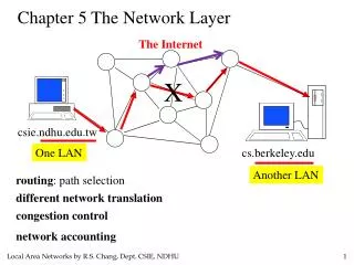
Chapter 5 The Network Layer. csie.ndhu.edu.tw. cs.berkeley.edu. routing : path selection. different network translation. congestion control. network accounting. 5. The Network Layer. 5.1 Network Layer Design Issues. 5.1.1 Services Provided to the Transport Layer. 5. The Network Layer.

Chapter 5 The Network Layer
E N D
Presentation Transcript
Chapter 5 The Network Layer csie.ndhu.edu.tw cs.berkeley.edu routing: path selection different network translation congestion control network accounting
5. The Network Layer 5.1 Network Layer Design Issues 5.1.1 Services Provided to the Transport Layer
5. The Network Layer 5.1 Network Layer Design Issues 5.1.1 Services Provided to the Transport Layer The network layer services have been designed with the following goals in mind: 1. The services should be independent of the subnet technology. 2. The transport layer should be shielded from the number, type, and topology of the subnets present. 3. The network addresses made available to the transport layer should use a uniform numbering plan, even across LANs and WANs.
5. The Network Layer 5.1 Network Layer Design Issues 5.1.1 Services Provided to the Transport Layer Two camps: 1. Connectionless services: Internet community (based on nearly 30 years of actual experience with a real, working computer network) 2. Connection-oriented services: telephone companies (based on 100 years of successful experience with the worldwide telephone system) The argument between connection-oriented and connectionless service really has to do with where to put the complexity (the subnet or the host).
5. The Network Layer 5.1 Network Layer Design Issues 5.1.1 Services Provided to the Transport Layer Supporters of connectionless service say: 1. User computing power has become cheap, so there is no reason not to put the complexity in the hosts. 2. The subnet is a major international investment that will last for decades, so it should not be cluttered up with features that may become obsolete quickly. 3. Some applications, such as digitized voice and real-time data collection may regard speedy delivery as much more important than accurate delivery. For example, the Internet TCP/IP protocol
5. The Network Layer 5.1 Network Layer Design Issues 5.1.1 Services Provided to the Transport Layer Supporters of connection-oriented service say: 1. Most users are not interested in running complex transport layer protocols in their machines. 2. Some services, such as real time audio and video are much easier to provide on top of a connection-oriented network layer. For example: Asynchronous Transfer Mode networks
5. The Network Layer 5.1 Network Layer Design Issues 5.1.2 Internal Organization of the Network Layer Virtual Circuits, in analogy with the physical circuits set up by the telephone system Datagrams, in analogy with telegrams
5. The Network Layer 5.1 Network Layer Design Issues 5.1.2 Internal Organization of the Network Layer
IP datagram: 223.1.1.1 223.1.2.1 E B A 223.1.1.2 source IP addr 223.1.2.9 misc fields dest IP addr 223.1.1.4 data 223.1.2.2 223.1.3.27 223.1.1.3 223.1.3.2 223.1.3.1 Dest. Net. next router Nhops 223.1.1 1 223.1.2 223.1.1.4 2 223.1.3 223.1.1.4 2 Getting a datagram from source to dest. routing table in A • datagram remains unchanged, as it travels source to destination • addr fields of interest here
223.1.1.1 223.1.2.1 A E B 223.1.1.2 223.1.2.9 223.1.1.4 223.1.2.2 223.1.3.27 223.1.1.3 223.1.3.2 223.1.3.1 Dest. Net. next router Nhops 223.1.1 1 223.1.2 223.1.1.4 2 223.1.3 223.1.1.4 2 Getting a datagram from source to dest. misc fields data 223.1.1.1 223.1.1.3 Starting at A, given IP datagram addressed to B: • look up net. address of B • find B is on same net. as A • link layer will send datagram directly to B inside link-layer frame • B and A are directly connected
223.1.1.1 223.1.2.1 A E B 223.1.1.2 223.1.2.9 223.1.1.4 223.1.2.2 223.1.3.27 223.1.1.3 223.1.3.2 223.1.3.1 Dest. Net. next router Nhops 223.1.1 1 223.1.2 223.1.1.4 2 223.1.3 223.1.1.4 2 Getting a datagram from source to dest. misc fields data 223.1.1.1 223.1.2.3 Starting at A, dest. E: • look up network address of E • E on different network • A, E not directly attached • routing table: next hop router to E is 223.1.1.4 • link layer sends datagram to router 223.1.1.4 inside link-layer frame • datagram arrives at 223.1.1.4 • continued…..
Dest. next 223.1.1.1 network router Nhops interface 223.1.2.1 E B A 223.1.1 - 1 223.1.1.4 223.1.1.2 223.1.2 - 1 223.1.2.9 223.1.2.9 223.1.1.4 223.1.3 - 1 223.1.3.27 223.1.2.2 223.1.3.27 223.1.1.3 223.1.3.2 223.1.3.1 Getting a datagram from source to dest. misc fields data 223.1.1.1 223.1.2.3 Arriving at 223.1.4, destined for 223.1.2.2 • look up network address of E • E on same network as router’s interface 223.1.2.9 • router, E directly attached • link layer sends datagram to 223.1.2.2 inside link-layer frame via interface 223.1.2.9 • datagram arrives at 223.1.2.2!!! (hooray!)
5. The Network Layer 5.1 Network Layer Design Issues 5.1.2 Internal Organization of the Network Layer
5. The Network Layer 5.2 Routing Algorithms routing algorithm: determine the route and maintain the routing table desired properties for a routing algorithm: 1. correctness 2. simplicity 1. robustness with respect to failures and changing conditions 2. stability of the routing decisions 3. fairness of the resource allocation 4. optimality of the packet travel times
5. The Network Layer 5.2 Routing Algorithms Fairness and optimality are often contradictory goals.
5. The Network Layer 5.2 Routing Algorithms What is it that we seek to optimize? Minimizing mean packet delay is an obvious candidate, but so is maximizing total network throughput. Furthermore, these two goals are also in conflict, since operating any queuing system near capacity implied a long queuing delay. As a compromise, many networks attempt to minimize the number of hops a packet must make, because reducing the number of hops tends to improve the delay and also reduce the amount of bandwidth consumed, which tends to improve the throughput as well.
5. The Network Layer 5.2 Routing Algorithms Static (nonadaptive) Routing The routing table is not changed according to network conditions. adaptive routing centralized routing: one node calculates the routing table isolated routing: do not exchange information with other node distributed routing: node exchanges information and makes routing decisions by itself
5. The Network Layer 5.2 Routing Algorithms 5.2.1 The Optimality Principle The optimality principle states that if router J is on the optimal path from router I to router K, then the routes from I to J and from J to K are also optimal. As a direct consequence of the optimality principle, we can see that the set of optimal routes from all sources to a given destination form a tree rooted at the destination. Such a tree is called a sink tree.
5. The Network Layer 5.2 Routing Algorithms 5.2.1 The Optimality Principle A sink tree for router B
5. The Network Layer 5.2 Routing Algorithms 5.2.1 The Optimality Principle A sink tree does not contain any loops, so each packet will be delivered within a finite and bounded number of hops. In practice, life is not quite this easy. Links and routers can go down and come back up during operation, so different routers may have different ideas about the current topology. Also, we have quietly finessed the issue of whether each router has to individually acquire the information on which to base its sink tree computation, or whether this information is collected by some other means.
5. The Network Layer 5.2 Routing Algorithms 5.2.2 Shortest Path Routing To compute the shortest path from A to D: Dijkstra’s algorithm
5. The Network Layer 5.2 Routing Algorithms 5.2.2 Shortest Path Routing To compute the shortest path from A to D
5. The Network Layer 5.2 Routing Algorithms 5.2.2 Shortest Path Routing To compute the shortest path from A to D
5. The Network Layer 5.2 Routing Algorithms 5.2.2 Shortest Path Routing To compute the shortest path from A to D
5. The Network Layer 5.2 Routing Algorithms 5.2.2 Shortest Path Routing To compute the shortest path from A to D
5. The Network Layer 5.2 Routing Algorithms 5.2.2 Shortest Path Routing To compute the shortest path from A to D
5. The Network Layer 5.2 Routing Algorithms 5.2.3 Flooding P Transmit a copy of each packet it receives on every one of its transmission links flooding P P P advantages: robust, simple, broadcasting, discovery disadvantages: use too much resource 1. hop count 2. time stamp How to curb the flooding: A variation of flooding that is slightly more practical is selective flooding. In this algorithm the routers do not send every incoming packet out on every line, only on those lines that are going approximately in the right direction.
5. The Network Layer 5.2 Routing Algorithms 5.2.4 Flow-Based Routing A subnet with line capacity shown in kbps
5. The Network Layer 5.2 Routing Algorithms 5.2.4 Flow-Based Routing The traffic in packets/sec and the routing matrix
5. The Network Layer 5.2 Routing Algorithms delay 5.2.4 Flow-Based Routing 800 bits packet
5. The Network Layer 5.2 Routing Algorithms 5.2.5 Distance Vector Routing Distance vector routing algorithms operate by having each router maintain a table (i.e., a vector) giving the best known distance to each destination and which line to use to get there. These tables are updated by exchanging information with the neighbors. E.g.: Routing table for Router A Destination cost(delay, distance, …) via ... B 10 B C B 12 D
5. The Network Layer 5.2 Routing Algorithms 5.2.5 Distance Vector Routing It was the original ARPANET routing algorithm and was also used in the Internet under the name RIP (Routing Information Protocol) and in early versions of DECnet and Novell’s IPX. AppleTalk and Cisco routers use improved distance vector protocols. Once every T msec each router sends to each neighbor a list of its estimate delays to each destination. It also receives a similar list from each neighbor.
5. The Network Layer 5.2 Routing Algorithms 5.2.5 Distance Vector Routing
5. The Network Layer 5.2 Routing Algorithms 5.2.5 Distance Vector Routing The count-to-infinity problem A is down Then A comes up. The good news spreads quickly.
5. The Network Layer 5.2 Routing Algorithms Then A comes down. The bad news travels slowly. 5.2.5 Distance Vector Routing The count-to-infinity problem A is up
5. The Network Layer 5.2 Routing Algorithms 5.2.5 Distance Vector Routing The count-to-infinity problem It should be clear why bad news travels slowly: no router ever has a value more than one higher than the minimum of all its neighbors. Gradually, all the routers work their way up to infinity, but the number of exchanges required depends on the numerical value used for infinity. For this reason, it is wise to set infinity to the longest path plus 1 (if using hop count as metric). If the metric is time delay, there is no well-defined upper bound, so a high value is needed to prevent a path with a long delay from being treated as down.
5. The Network Layer 5.2 Routing Algorithms 5.2.5 Distance Vector Routing The Split Horizon Hack Many ad hoc solutions to the count-to-infinity problem have been proposed in the literature, each one more complicated and less useful than the one before it. We will describe just one of them and tell why it, too, fails. The split horizon algorithm works the same way as distance vector routing, except that the distance to X is not reported on the line that packets for X are sent on (actually, it is reported as infinity).
5. The Network Layer 5.2 Routing Algorithms 5.2.5 Distance Vector Routing The Split Horizon Hack 1 2 3 4 inf 2 3 4 inf inf 3 4 inf inf inf 4 inf inf inf inf inf=infinity
5. The Network Layer 5.2 Routing Algorithms 5.2.5 Distance Vector Routing The Split Horizon Hack When CD line goes down. A thinks it has a path to D through B and B thinks it has a path to D through A. A and B will count to infinity.
5. The Network Layer 5.2 Routing Algorithms 5.2.6 Link State Routing Distance vector routing was used in the ARPANET until 1979, when it was replaced by link state routing. Two primary reasons caused its demise. First, since the delay metric was queue length, it did not take line bandwidth into account when choosing routes. Second, the algorithm often took too long to converge, even with tricks like split horizon. For these reasons, it was replaced by an entirely new algorithm now called link state routing.
5. The Network Layer 5.2 Routing Algorithms 5.2.6 Link State Routing The idea behind link state routing is simple and can be stated as five parts. Each router must: 1. Discover its neighbors and learn their network addresses. 2. Measure the delay or cost to each of its neighbors. 3. Construct a packet telling all it has just learned. 4. Send this packet to all other routers. 5. Compute the shortest path to every other router.
5. The Network Layer 5.2 Routing Algorithms 5.2.6 Link State Routing Distance vector routing differs significantly from the link state routing. With link state algorithms, routers share only the identity of their neighbors, but they flood this information through the entire network. Distance vector algorithms adopt an opposite approach. Routers periodically share knowledge of the entire network, but only with their neighbors.
5. The Network Layer 5.2 Routing Algorithms 5.2.6 Link State Routing Learning about the Neighbors When a router is booted, its first task is to learn who its neighbor are. It accomplishes this goal be sending a special HELLO packet on each point-to-point line. The router on the other end is expected to send back a reply telling who it is. When two or more routers are connected by a LAN, the situation is slighted more complicated. One way to model the LAN is to consider it as a node itself.
5. The Network Layer 5.2 Routing Algorithms 5.2.6 Link State Routing Learning about the Neighbors An artificial node
5. The Network Layer 5.2 Routing Algorithms 5.2.6 Link State Routing Measuring Line Cost The link state routing algorithm requires each router to know, or at least have a reasonable estimate, of the delay to each of its neighbors. The most direct way to determine this delay is to send a special ECHO packet over the line that the other side is required to send back immediately. By measuring the round-trip time and dividing it by two, the sending router can get a reasonable estimate of the delay.
5. The Network Layer 5.2 Routing Algorithms 5.2.6 Link State Routing Measuring Line Cost An interesting issue is whether or not to take the load into account when measuring the delay. To factor the load in, the round-trip timer must be started when the ECHO packet is queued. To ignore the load, the timer should be started when the ECHO packet reaches the front of the queue.
5. The Network Layer Including load in delay calculation: can use the best line, but may lead to routing table oscillating. 5.2 Routing Algorithms 5.2.6 Link State Routing Measuring Line Cost Same bandwidth on the two links
5. The Network Layer 5.2 Routing Algorithms 5.2.6 Link State Routing Building Link State Packets Building the link state packets is easy. The hard part is determining when to build them. 1) Periodically 2) When some significant event occurs, such as a line or neighbor going down or coming back up.
5. The Network Layer 5.2 Routing Algorithms 5.2.6 Link State Routing Distributing the Link State Packets The trickiest part of the algorithm is distributing the link state packets reliably. As the packets are distributed and installed, the routers getting the first ones will change their routes. Consequently, the different routers may be using different versions of the topology, which can lead to inconsistencies, loops, unreachable machines, and other problems. The fundamental idea is to use flooding to distribute the link state packets.
5. The Network Layer 5.2 Routing Algorithms 5.2.6 Link State Routing Distributing the Link State Packets To keep the flood in check, each packet contains a sequence number that is incremented for each new packet sent. Routers keep track of all the (source router, sequence) pairs they see. When a new link state packet comes in, it is checked against the list of packets already seen. 1. If new: forward on all lines except the one it arrived on 2. If duplicate or old packet: discard 3. If a packet with a sequence number lower than the highest one seen so far, it’s rejected as being obsolote.