Topic 2 Lecture 13
Topic 2 Lecture 13. Isoquants, the Short-run production function, Marginal product of labour, and firm’s costs. Production isoquants and the MRTS A household consumes x and y and derives Utility. x and y are inputs and utility is an output.

Topic 2 Lecture 13
E N D
Presentation Transcript
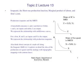
Topic 2 Lecture 13 • Isoquants, the Short-run production function, Marginal product of labour, and firm’s costs. • Production isoquants and the MRTS • A household consumes x and y and derives Utility. • x and y are inputs and utility is an output. • We represent the relationship with indifference curves. • For a firm, K and L are inputs and X is the output. • We represent the relationship with production isoquants. • Also think about concept of a trade-off along • the Isoquant. B&B ch. 6 explores in detail the idea of the • production iso-quant (and the analogy with topographic • mappings with contour lines). Slope of IC is MRS U = U(X, Y) y U x K Slope of Iso-quant is MRTS X = X(K, L) X L Robin Naylor, Department of Economics, Warwick
Topic 2: Lecture 13 Think about a 3-D map of a mountain. The mountain can be represented in a contour map (which is a view from above). The analogy is with an iso-quant diagram. The axes are K and L. We can consider how different output levels can be achieved by changing K and/or L. The mountain can also be shown in profile (the view from one side). If we view the mountain from the south, we can see how height varies along its east-west profile from a particular southern viewpoint – but are unable to discern how height changes along the south-north dimension. The analogy is with the short-run production function, which shows how output varies with L for a particular level of K. As my focus is on the short-run (in which K is constant) the production function is the diagram I am most interested in. Robin Naylor, Department of Economics, Warwick
Topic 2 Lecture 13 In the short-run, K is fixed: X The short-run production function: X = X(L) L In the short-run the firm can vary only Labour inputs. Labour is variable and so the costs of employing Labour are variable. The amount of Capital, and hence the costs of employing Capital, are Fixed. Robin Naylor, Department of Economics, Warwick
Topic 2 Lecture 13 X The short-run production function: X = X(L) L Assumption: The slope of the short-run production function is positive, but it is decreasing . . . (Note – if you want to relate this to the iso-quant diagrams, see B&B page 233, Figure 6.19) Robin Naylor, Department of Economics, Warwick
Topic 2 Lecture 13 X The short-run production function: X = X(L) L Slope of X=X(L) In terms of Economics, what is the slope of X(L)? L Robin Naylor, Department of Economics, Warwick
Topic 2 Lecture 13 X The short-run production function: X = X(L) dX dL L MPPL L Robin Naylor, Department of Economics, Warwick
Topic 2 Lecture 13 Robin Naylor, Department of Economics, Warwick
Topic 2 Lecture 13 X X = X(L) DRL L From the shape of the Short-run production function, we can infer the shape of the firm’s MPPL curve, as we have seen, and also: (i) the shape of the firm’s Short-run Marginal Cost (SMC) curve and (ii) the shape of the firm’s Short-run Total Variable Cost (STVC) curve. (For now, we are considering only the firm’s Variable Costs.) Robin Naylor, Department of Economics, Warwick
Topic 2 Lecture 13 X X = X(L) From the shape of the Short-run production function, we can infer the shape of the firm’s MPPL curve and also: (i) the shape of the firm’s Short-run Marginal Cost (SMC) curve DRL L Robin Naylor, Department of Economics, Warwick
Topic 2 Lecture 13 X DRL X = X(L) From the shape of the Short-run production function, we can infer the shape of the firm’s MPPL curve and also: (i) the shape of the firm’s Short-run Marginal Cost (SMC) curve dX2 X2 dX1 X1 L SMC What is the Marginal Cost of raising output by one unit from X1. . . . ? = ? X X1 X2 Robin Naylor, Department of Economics, Warwick
Topic 2 Lecture 13 X DRL X = X(L) From the shape of the Short-run production function, we can infer the shape of the firm’s MPPL curve and also: (i) the shape of the firm’s Short-run Marginal Cost (SMC) curve dX2 X2 dX1 X1 L dL1 SMC What is the Marginal Cost of raising output by one unit from X2 . . . . ? = ? X X1 X2 Robin Naylor, Department of Economics, Warwick
Topic 2 Lecture 13 X DRL X = X(L) From the shape of the Short-run production function, we can infer the shape of the firm’s MPPL curve and also: (i) the shape of the firm’s Short-run Marginal Cost (SMC) curve dX2 X2 dX1 X1 L dL1 dL2 SMC What is the Marginal Cost of raising output by one unit from X2 . . . . ? = ? X X1 X2 Robin Naylor, Department of Economics, Warwick
Topic 2 Lecture 13 X DRL X = X(L) From the shape of the Short-run production function, we can infer the shape of the firm’s MPPL curve and also: (i) the shape of the firm’s Short-run Marginal Cost (SMC) curve dX2 X2 dX1 X1 L dL1 dL2 SMC So: SMC(X1) = w.dL1 and SMC(X2) = w.dL2 => Thus, SMC1<SMC2. X X1 X2 Robin Naylor, Department of Economics, Warwick
Topic 2 Lecture 13 X DRL X = X(L) From the shape of the Short-run production function, we can infer the shape of the firm’s MPPL curve and also: (i) the shape of the firm’s Short-run Marginal Cost (SMC) curve dX2 X2 dX1 X1 L dL1 dL2 SMC So: SMC(X1) = w.dL1 and SMC(X2) = w.dL2 => Thus, SMC1<SMC2. SMC2 SMC1 X X1 X2 Robin Naylor, Department of Economics, Warwick
Topic 2 Lecture 13 X DRL X = X(L) From the shape of the Short-run production function, we can infer the shape of the firm’s MPPL curve and also: (i) the shape of the firm’s Short-run Marginal Cost (SMC) curve dX2 X2 dX1 X1 L dL1 dL2 SMC So: SMC(X1) = w.dL1 and SMC(X2) = w.dL2 => Thus, SMC1<SMC2. SMC SMC2 SMC1 X X1 X2 Robin Naylor, Department of Economics, Warwick
Topic 2 Lecture 13 X DRL X = X(L) Three ways of showing the same thing . . . . . . DRL dX2 X2 dX1 X1 dL1 dL2 MPPL SMC SMC DRL DRL SMC2 SMC1 MPPL L X X1 X2 Robin Naylor, Department of Economics, Warwick
Topic 2 Lecture 13 X STVC X = X(L) ? DRL X L SMC SMC DRL X From the shape of the Short-run production function, we can also infer : (ii) the shape of the firm’s Short-run Total Variable Cost (STVC) curve. Robin Naylor, Department of Economics, Warwick
Topic 2 Lecture 13 X STVC X = X(L) ? DRL DRL X L SMC The STVC shows us what happens to the firm’s total Labour costs as output (and hence labour employment) increases. STVC certainly increasing: but is it linear? Or is it getting steeper? Or flatter? As SMC is rising under DRL, it follows that STVC is getting steeper: Why? SMC DRL X Robin Naylor, Department of Economics, Warwick
Topic 2 Lecture 13 X STVC STVC X = X(L) DRL DRL DRL X L SMC As SMC is rising under DRL, it follows that STVC is getting steeper: Why? Mathematically, what is the relationship between STVC and SMC? SMC DRL X Robin Naylor, Department of Economics, Warwick
Topic 2 Lecture 13 X STVC STVC X = X(L) DRL DRL DRL X MPPL L SMC SMC DRL MPPL DRL X L Robin Naylor, Department of Economics, Warwick
Topic 2 Lecture 13 X STVC X = X(L) ? IRL IRL X MPPL L SMC ? ? IRL IRL X L Robin Naylor, Department of Economics, Warwick
Topic 2 Lecture 13 X STVC X = X(L) ? CRL CRL X MPPL L SMC ? ? CRL CRL X L Robin Naylor, Department of Economics, Warwick
Topic 2 Lecture 13 X STVC X = X(L) DRL ? IRL X MPPL L SMC ? ? X L Robin Naylor, Department of Economics, Warwick
Topic 2: Lecture 13 Now read B&B 4th Ed., Chapter 6 on Inputs and Production Functions and Chapter 7 on Cost-minimisation and Chapter 8 on Cost Curves. If you want to follow B&B in the same order as the material in lectures, you might start with section 6.3 on p. 210. Read as far as p. 219 and then go back to pp. 201-210. There is no need to study pp. 220-239 (but don’t let me stop you . . . These pages will deepen your understanding). Chapter 7 goes into more detail than you need to follow the lecture material. You should focus on pp. 245-254, 270-271. In lectures, I avoid the need to use the idea of the iso-cost line – but Chapter 8 will be easier to follow if you make some effort to follow the idea of the iso-cost line in Chapter 7. In Chapter 8, you should focus on pp. 292-310. Robin Naylor, Department of Economics, Warwick