Population Ecology

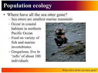
1. Population Ecology Reading: Freeman, Chapter 52

2. Every species has a geographic range • A geographic range describes where individuals of a species might potentially be located. • In the United states, most species have a range of 4-24 states. • Cosmopolitan species are an extreme, they are worldwide in distribution. • Endemic species are found in only a small, restricted area, they represent the other side of the spectrum.

3. This is the geographic range of a species of damselfly. campus.greenmtn.edu/dept/NS/Dragonfly/Vermont

4. Factors Determining the Geographic Range of a Species • History • Biological Tolerances • Other Species • A combination of the above

5. Historical Factors Determining Range: Example • Many species have what is called a “Gondwanan” distribution. They occur in the Southern continents of Australia, South Africa, South America, and sometimes India. • These places are far away from each other now, but 150 million years ago, they were all linked together in a massive continent. • Examples number in the thousands, across many different types of species, including the rattite birds, the bee family colettidae, and the southern beech tree, Nothofagus sp.

6. The geographic ranges of various ratite birds

9. No species are truly ubiquitous, in the sense that all species are restricted to a particular habitat. • Suitable habitats tend to be clustered within the geographic range of a population, therefore, most species are composed of discontinuous groups called populations. • Clearly, the boundaries between populations can be somewhat subjective. • What constitutes a population depends upon the species in question, but in general, members of a population interact, mate, and compete with each other much more frequently than members of different populations.

10. Populations are groups of individuals of the same species living in the same place • Individuals within a population occupy the same general area, rely on the same resources, and are influenced by the same general environmental conditions. • Most of the interaction, including sexual reproduction, between individuals of a species is among members of the same population.

11. Some populations move • A single population of salmon may spawn upstream in a river of the Pacific Northwest, and return to the ocean to feed and grow. • Most of the interaction between individuals and exchange of alleles, occurs among individuals nesting in the same stream. • Likewise, a population of monarch butterflies may migrate, en masse, to over-wintering grounds in Mexico for the winter, returning to the Midwest to reproduce during the summer (although no single individual makes the whole trip).

13. Populations have certain emergent properties • These properties are consequences of the way an organism interacts with the environment, and with other organisms, and influence its evolution. • Size • Density • Patterns of Dispersion • Age Structure • Spatial Structure • Sex Ratio • Variability

14. Size • Simply the number of individuals in the population at any given time. Sometimes called abundance.

15. Density • The number of individuals in the population per unit area or unit volume. • For many organisms, it is the density of a population rather than its actual numbers, that exerts a real effect on the organism.

16. Example Problem • There are 10,400 mice living in a 1000m x 1000m field. What is the density of this population?

17. Answer • The area of the field is 1,000,000 square meters (m2). • The density of mice is therefore 10,400 mice/1,000,000m2=.0104/m2.

18. Patterns of Dispersion • Populations follow into three different patterns of dispersion, generally. • Clumped • Regular • Random

19. Clumping is probably the most common situation.Sometimes clumping occurs because some areas of habitat are more suitable than others • i.e., Plethodon sp. salamanders are found clumped under fallen logs in the forest • the night lizard Xantusia sp. is found clumped within fallen Joshua trees in the Mojave desert

20. Sometimes species clump for other reasons. • Plants often clump because their seeds fall close to the parent plant or because their seeds only germinate in certain environments. Impatiens capensis seeds are heavy and usually fall close to the parent plant-this species grows in dense stands. • Species may clump for safety, or social reasons. Ground nesting bees Halictus sp. prefer to nest in the presence of other bees, forming aggregations of solitary nests

21. Random distribution • This pattern occurs in the absence of strong attraction or repulsion among individuals. • It is uncommon. • The trees of some forest species are randomly distributed within areas of suitable habitat. • For example, fig trees in the amazon rain forest. This random distribution might be due to seed dispersal by bats.

22. Regular Distribution • This generally happens because of interactions between individuals in the population. • Competition: Creosote bushes in the Mojave desert are uniformly distributed because competition for water among the root systems of different plants prohibits the establishment of individuals that are too close to others. • Territoriality: The desert lizard Uta sp. maintains somewhat regular distribution via fighting and territorial behavior • Human Intervention: I.e., the spacing of crops.

23. Spatial Structure • The scale matters a great deal in describing the spatial distribution of a species. • A species may be clumped on the large scale, but evenly distributed on a finer scale. • Example: Ground nesting wasps, Sphex sp. are clustered in areas of suitable nesting substrate (packed sand). Within these areas, their nests are evenly distributed because of aggressive interactions.

24. Age structure • This is the relative number of individuals at different ages.

25. Sex ratio • Sex ratio is the proportion of individuals of each sex.The number of females is more important in the overall growth rate of populations • Examples: elk; fewer males of reproductive age than females; males breed with more than one female. • Wasps: Melittobia sp. may have as many as a hundred females per male. These males never leave the nest and mate with their sisters. Population growth is essentially independent of the number of males.

26. Variability is differences among individuals in the population. • Most populations show differences among individuals. • Some variation has a genetic basis. • Other variation is largely environmental. • In many cases, variability is caused by both genes and the environment. • Sexual Dimorphism is when the two sexes differ greatly in appearance. • Metamorphosis is when individuals differ in appearance because of a dramatic transformation as they age.

27. It is a fundamental characteristic of living things that all organisms reproduce. • Every species is capable of population growth under some set of possible conditions

28. DemographicProcesses • Birth (Natality) • Death (Mortality) • Immigration • Emigration

29. Exponential Growth • This is probably the best, simple, model of population growth…it predicts the rate of growth, or decay, of any population where the per capita rates of growth and death are constant over time. • In exponential growth models, births deaths, emigration and immigration take place continuously • This is a good approximation for the growth of most biological populations • i.e., human populations grow exponentially when resources are plentiful

30. DN/DT=bN-dN • Where: • b is the per capita birth rate • d is the per capita death rate • ignoring immigration and emmigration. • dN/dT=rN (define r as the instantaneous population growth rate; r=b-d) • you can integrate this to get the exponential growth formula that follows… • Note that we are assuming that there is no emigration or immigration.

31. Exponential growth formula • N(t)=N0ert • where r is the exponential growth parameter • N0 is the starting population • t is the time elapsed • r=0 if the population is constant, r>0 if population is increasing, r<0 if the population is decreasing.

32. Example problem • The human population of the earth is growing at approximately 1.8%per year. • The population at the start of 2001 was approximately 6 billion. • If nothing were to slow the rate of population growth, what would the population be in the year 2101?

33. Answer • N(t)=N0ert • r= .018 • t=100 years • N0=6 billion • N(100)=N0ert • N(100)=6x109ert =6x109*e1.8 • N(100)= 6x109*6.04= 36.3 billion

34. Limits to Growth • No population can continue growing forever. • Even organism that reproduce very slowly, such as elephants, rhinos, whales, and humans, would outstrip their resources if they reproduced indefinitely.

35. Carrying Capacity • Populations grow until one or several limiting resources become rare enough to inhibit reproduction so that the population no longer grows. • The limiting resource can be light, water, nesting sites, prey, nutrients or other factors. • Eventually, every population reaches its carrying capacity, this is the maximum number of individuals a given environment can sustain.

36. Logistic Growth Model • The logistic growth model accounts for carrying capacity. • K= Carrying Capacity, this is the maximum number of individuals that the population can sustain. • N=The Number of individuals in the population at a given time • rmaxis the maximum population growth rate • dN/dT=rmaxN(K-N)/K • Question: What is dN/dT when N=K?

37. Answer • When N=K, dN/dT=0 • Likewise, when N is small, • dN/dT =approximately rmax • When N>K the population declines.

39. How Well Does the Logistic Model Fit Actual Populations? • For laboratory populations of Paramecia, crustaceans, etc.., the logistic provides a pretty good fit. • For actual populations, the logistic does not provide such a good fit. • There are usually other factors involved. • One factor: lag time is the time it takes between reaching carrying capacity and the slowdown in reproduction.

40. Demography • Demography is the study of the age structure and growth of populations, especially as it relates to the births and deaths of individuals. • The study of human mortality goes back a long way, to the Middle Ages and the early Renaissance. Thomas Malthus was a rather famous early demographer/economist. In his Essay on the Principal of population, 1798, he was the first to reach the conclusion that human populations tended to grow until they outstripped their available food supply.

41. Counting Individuals • Complete enumeration: count every individual in the population • Sample the Population: • count individuals in many small portions of the area (e.g., quadrats) then calculate density • mark and recapture • index of relative abundance (e.g., pheremone baited insect traps)

42. Mark-Recapture Example • A population of bats lives under a bridge in Texas. On Monday, 50 bats are netted and marked with ear tags. On Tuesday, the same researchers return and net 100 bats. Of these, 13 are marked. • How many bats live under the bridge?

43. Answer: • First Sample = Marked Recaptures • TOTAL POPTotal Recaptures • 50/T=13/100 (where T is the population of bats under the bridge) • multiply both sides by 100T • 5000=13T • T=385

44. Life Tables • A person’s chance of death is of tremendous interest to a person selling life insurance. Life tables are based on the actuarial tables insurance companies keep. • By tabulating deaths, causes of death, and ages of death, it is obvious that a person’s chance of dying is not constant over time. For humans, it increases as we get past a certain age. • Biologists have adopted Life Tables and applied them to other species.

45. Constructing a Life Table • A Cohort is a group of organisms born at the same time. • S(0) is the number of individuals born into the cohort. S(x) is the number of individuals alive at the start of interval x. • D(x) is the number of individuals dying during interval x. • l(x) is the proportion of individuals alive at the start of interval x. l(x)=S(x)/S(0) • m(x) is the expected number of female offspring born to a female during interval x.

46. Life Table for a Field Grasshopper • X s(x) d(x) l(x) m(x) l(x)*m(x) • eggs 0 44000 40487 1.000 0 0 • Instar I 1 3513 984 .080 0 0 • Instar II 2 2519 597 .057 0 0 • Instar III 3 1922 461 .044 0 0 • Instar IV 4 1461 161 .033 0 0 • Imago 5 1300 1300 .030 17 .51 • R0=.51 • adapted from Richards and Waloff, 1954

47. Survivorship Curves • A survivorship curve traces the decline of a group of newborns over time. • Survivorship curves plot the probability of surviving to a certain age for a representative member of the population

48. Types of Survivorship Curves • Type I: A convex curve. Most individuals live to adulthood with most mortality occurring during old age. I.e., humans, red deer, elephants. • Type II: A straight line. An individual’s chance of dying is independent of its age. I.e., small birds and mammals. • Type III: A concave curve, few individuals live to adulthood, with the chance of dying decreasing with age. I.e., oysters, redwood trees, snapping turtles.

49. http://www.io.uwinnipeg.ca/~simmons/1116/