Download
1 / 78
930 likes | 1.53k Vues
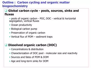
Outline : Carbon cycling and organic matter biogeochemistry. Global carbon cycle - pools, sources, sinks and fluxes pools of organic carbon - POC, DOC - vertical & horizontal segregation, vertical fluxes Ocean productivity Biological carbon pump Preservation of organic carbon

E N D
Outline : Carbon cycling and organic matter biogeochemistry • Global carbon cycle - pools, sources, sinks and fluxes • pools of organic carbon - POC, DOC - vertical & horizontal segregation, vertical fluxes • Ocean productivity • Biological carbon pump • Preservation of organic carbon • Vertical flux of POM – sediment traps • Dissolved organic carbon (DOC) • Concentrations & distribution • Characterization of DOC pool - molecular size and reactivity • Sources and fates of POM & DOM • Age and long-term sinks for DOM
Operational pools of carbon in seawater • POM - particulate organic matter (includes not only carbon but also H, O, N, P, S etc) • DOM - dissolved organic matter (about 50% C by weight) • POC - particulate organic carbon (refers only to the carbon) • DOC - dissolved organic carbon • PIC – Particulate inorganic carbon (CaCO3) • DIC - dissolved inorganic carbon (all forms) • Organic nutrient pools • PON & POP (the pools of N & P that are bound in organic particles larger than the operational cut-off) • DON & DOP - (the pools of N & P that are bound in organic matter that passes through the operational cut-off filter) All pools are operational! (depend on selected criteria for filtration)
Organic particle size continuum 0.4-0.2 µm filtration cut-off
Organic carbon = Reduced carbon • Includes all carbon other than CO2, HCO3-, H2CO3, CO, CO32-, and carbonate minerals • Includes hydrocarbons CH4, CH3-CH3 etc & black carbon. • Nearly all reduced carbon is biogenic. However, some chemical/geochemical alteration of OM takes place, petroleum and natural gas formation being notable examples. • Because organic matter is mainly biogenic it typically contains not only reduced carbon but also some H, O, N, P and S etc.
Global Carbon reservoirs and exchanges (Figure based on Libes; data from Table 11.1 in Emerson & Hedges) pools in 1015 gC (boxes) fluxes in 1015 gC y-1 (arrows) Atmospheric CO2 784 Terrestrial biota 600 River DIC 0.5 Exchange 90 Soil & detritus 1500 Net export from surface 8-15 Ocean DIC 38,000 Marine biota 1-2 Detrital POC 30 DOC 700 0.2 Sedimentary reservoirs are huge! Organic sediments 10,000,000 Fossil fuels 3577 Limestone & dolomite 50,000,000
Most organic carbon in the sea is dissolved or colloidal. • Biomass pools are very small Operationally-dissolved Dissolved and Colloidal materials are operationally Dissolved
Sources of organic matter to the open oceans % of total Primary production Phytoplankton 84.4 Macrophytes 6.2 Rivers 3.65 Groundwater 0.3 Atmospheric input 5.45 Rivers are a small source of organic matter to open ocean! Based on Table 9.1 in Millero, 2006
Ocean Net Primary Production in different trophic regimes % of Ocean NPP Oligotrophic < 0.1 11.0 22.7 (<100 gC m-2 y-1) 56.5 Mesotrophic 0.1 -1.0 27.4 (100-300 gC m-2 y-1) Eutrophic > 1.0 9.1 18.7 (300-500 gC m-2 y-1) Macrophytes - 1.0 2.1 Total ocean production = 48.5 Total terrestrial production = 56.4 Total global production = 104.9
Global primary productivity pattern as deduced from satellite imagery Behrenfeld et al 2006. Nature 444: • Considerations: • Depth distribution i.e. euphotic depth • Seasonal variations, esp. in polar regions • Interannual variations Oceanic/oligotrophic areas– dominated by picoplankton < 2 μm Upwelling, coastal & temperate areas have larger phytoplankton (> 2 μm) as major primary producers
Temporal changes in global average Chlorophyll anomaly and Net Primary Productivity (NPP) anomaly. 1997-98 was a strong El Nino year which reduced NPP. Rapid recovery ensued, with slow decline thereafter. Behrenfeld et al 2006. Nature 444:
The Biological Carbon Pump Exporting carbon below the pycnocline CO2 (g) CO2 (aq) + H2O <=> H2CO3 <=> H+ + HCO3- <=> H+ + CO32- Air Sea Euphotic zone calcification Photosynthesis Pycnocline sinking Upwelling of high DIC, high pCO2 water POM CaCO3 Some DOM DIC & alkalinity CaCO3-rich sediment above CCD No preservation of CaCO3 below CCD CO2 Deep Sea respiration spreading Alkalinity POM CCD Ridge crest CaCO3 dissolution Carbon burial & preservation as POM and CaCO3 Non-carbonate sediment carbonates
Export Production per year Falkowski et al., 1998. Science 298:
Flux of organic matter decreases exponentially with depth : POMflux(z) = POMflux (100)(z/100)-0.858 Where POMflux(100) is the downward flux at the base of the euphotic zone (100 m), and POMflux(z) is the flux of organic carbon at depth (z) measured with sediment traps. At 5000 meters, the flux is only 3.5% of that at the base of the euphotic zone! Very little organic matter (POM) reaches the deep ocean – and what does reach the bottom is lower quality Data for the figure of Bishop et al came from Martin et al. 1987 Vertical flux of POM is via dead phytoplankton, fecal pellets, molt shells, fragments, mucous feeding nets etc.
DOC export from surface ocean represents 8-18% of the total organic carbon export. Modeled DOC downward flux DOC/POC downward flux ratio Hansell et al., 2010
Sediment traps - particle interceptors Baffle to reduce hydrodynamic effects Poison or preservative Particle flux Base of euphotic zone 100-200 m 500 m Capture flux decreases exponentially with depth 1000 m 3000 m
Many different designs of sediment traps have been used Time series traps - rotating cylinders within trap collect for certain period of time 1-1.5 meters Large surface area trap for oceanic sampling
Diagram of an automated time-series sediment trap used in the Arabian Sea. A baffle at top keeps out large objects that would clog the funnel. The circular tray holds collection vials. On a preprogrammed schedule (every 5 days to 1 month), the instrument seals one vial and rotates the next one into place. Scientists retrieve the samples up to a year later to analyze the collected sediment. (courtesy Oceanus magazine, WHOI) http://www.whoi.edu/instruments/gallery.do?mainid=19737&iid=10286
What results do you expect for POM captured in a sediment trap array deployed over a full oceanic depth profile? • Quantity of POM? • Quality of POM - C:N, specific biomolecules?, 14C-content?
Three sediment trap designs. The original funnel design (moored trap) uses a large collection area to sample marine particulates that fall to great depths. Surface waters produce enough sediment so that traps there don’t require funnels. Neutrally buoyant, drifting sediment traps catch falling material instead of letting it sweep past in the current. Drawings are not to scale. Source: http://www.whoi.edu/instruments/gallery.do?mainid=19735&iid=10286
Joaquim Goes and his team deploy simple sediment traps in the Southern Ocean
WHOI scientists Ken Buesseler and Jim Valdes with one of the neutrally buoyant sediment traps they helped design. The central cylinder controls buoyancy and houses a satellite transmitter. The other tubes collect sediment as the trap drifts in currents at a predetermined depth, then snap shut before the trap returns to the surface. (Tom Kleindinst, WHOI) http://www.whoi.edu/instruments/gallery.do?mainid=19750&iid=10286
Much of the present global carbon burial (preservation) is in marine environments • Little organic carbon preservation in terrestrial soils except for high latitude peats. Terrestrial burial of OM has been more significant in the geological past (i.e. Carboniferous coal deposits) • Significance of Organic Carbon Burial • Burial and preservation of biogenic (reduced) carbon in sedimentary reservoirs removes atmospheric CO2 and allows excess O2 to remain in the atmosphere. • Burial of organic matter removes some nutrient elements and trace elements. • Carbon burial leads to petroleum, organic rich shales, & natural gas
The greater the overall sedimentation rate of particles, the greater the fraction of surface primary production delivered to sediments 100 Coastal areas – maximum of ~10% 10 1 Percent of primary production accumulated in the sediments 0.1 0.01 0.001 0.1 1 10 100 1000 Sediment accretion rate (cm per 1000 y) y = 0.028 x1.25 See Fig. 11.5 in Pilson for actual data graph >5000 m depth >2-5000 m depth >2000 m depth incl. Black Sea
Most burial nearshore on continental margins Burial will be a small fraction of the carbon delivered to the sediments. Most will be respired to CO2 and diffuse back to water column. Libes, Chapter 25
Reasons for high carbon burial on the continental margins: • high productivity - > high POM flux to benthos • high particle flux leading to faster burial rate - OM preservation tied directly to mineral surface area (see Keil et al. 94) • shallow depth - less organic matter degradation on descent • remineralization slower under anoxia - still a debatable issue.
Dissolved organic carbon - the largest pool of organic matter in seawater • Measured by converting DOC into CO2 via: • Wet-chemical oxidation • High temperature catalytic combustion • UV-oxidation • Sealed tube combustion DOC concentrations are 70-100 µM in surface waters of the open ocean, and 35-50 µ M at depth. Coastal waters can have much higher DOC
Surface ocean (30 m) DOC concentrations Dots are measured values, background color field is modeled Hansell et al., 2010
Deep ocean (3000 m) DOC concentrations decrease along ocean conveyor (meridional overturning circulation) Dots are measured values, background color field is modeled NADW starts with about 46 µM DOC The semi-labile fraction of DOC degrades during the long transit from North Atlantic to the Pacific. What is left (~34 M) is ultra-refractory since it survived the ~1000 y trip through the deep ocean. This DOC is present as background DOC in surface waters and has an average age of ~6000 years. Hansell et al., 2010
DOC Concentration (µM) C A B 0 D 1000 2000 Depth (m) 3000 4000 60 30 50 20 10 40 70 0 Labile DOC; Small pool; τ = hours to days Semi labile DOC; larger pool (25-30 µM) in sfc; τ = weeks to months Open ocean surface DOC concentration is about 70 µM. It is about 44 µM in the deep Sargasso and about 34 µM in the deep Pacific. Ultra-refractory DOC; τ = >6000 y Refractory DOC; τ = ~1000 years After Benner, 2002
400 DOC (µM) 75 0 36 0 Salinity DOC is generally conservative with salinity in estuaries Implies terrestrial DOC delivery to ocean – but most is lost on shelf (see next slide) Freshwater end-member In fact, some modification of riverine DOC takes place in estuaries, but conservative pattern still observed Seawater end-member ~80-100 µM
DOC concentration decreases away from shore Much of the DOC delivery to ocean is lost on the shelf, close to shore
Constituents of DOM • High molecular weight >5000 Da (includes colloids) • proteins • polysaccharides (mucus, structural polymers) • nucleic acids • some humic substances • Medium Molecular weight 500-5000 Da • humic substances (refractory) • oligopeptides, oligonucleotides • lipids • pigments • Low molecular weight < 500 Da • monomers (sugars, amino acids, fatty acids) • osmolytes (DMSP, betaines, polyols) • toxins, pheromones and other specialty chemicals See Chapter 22 in Libes for structures of organic compounds Mixed lability – some very refractory High lability Moderate lability
Examples of some polysaccharides that might be part of a semi-labile, high molecular weight pool of DOM. Pectin contains O-methoxy groups Chitin is an amino sugar, i.e. it contains N
Depolymerization - Polymer hydrolysis • Conversion of high molecular weight DOM or POM into low molecular weight DOM • Carried out primarily by bacteria but really a • consortium of microbes. • Proteins -> free amino acids & peptides by proteases • Polysaccharides to monosaccharides by glucosidases, chitinases, cellulases • Peptides to amino acids by peptidases • RNA or DNA to nucleotides by nucleases
Origin of labile DOM in seawater • Exudates - Amino acids, sugars, some high molecular weight labile polysaccharides - rapidly consumed • Death or lysis of cells - rapid uptake by bacteria • Sloppy feeding - leaking of phytoplankton cell contents • Digestion - Digestor theory. Jumars, Penry et al. Zooplankton maximize their organic matter assimilation by maximizing throughput not by being highly efficient. This results in considerable release of DOC from fecal pellets and zooplankton.
Marine Snow. • Agglomerated organic matter - amorphous aggregates • Enriched with bacteria and protozoans • possible low oxygen conditions • elevated nutrients • Still understudied. Some species of phytoplankton release mucilage i.e. Phaeocycstis sp. TEP - Transparent ExoPolymer. Is a form of marine snow Marine Snow or aggregates caused by surface phenomenon. Enrichment of OM at surfaces of bubbles, waves convergence zones. You can make snow in the lab by rotating filtered water samples in bottle. Snow, and DOC make, sea foam.
Phaeocystis globosa colony –cells embedded in mucous form spherical colony http://www.ifremer.fr/delec-en/projets/efflores%20phyto/phaeocystis/phaeocys.htm http://www.microscopy-uk.org.uk/mag/artapr01/foam.html Sea foam generated from Phaeocystis bloom in Dutch Wadden Sea
Blowing sea foam at Nags Head, North Carolina during Hurricane Sandy, October 2012 Nags Head, N.C. High winds blow sea foam into the air as a person walks across Jeanette's Pier in Nags Head, N.C., Sunday, Oct. 28, 2012 as wind and rain from Hurricane Sandy move into the area. Governors from North Carolina, where steady rains were whipped by gusting winds Saturday night, to Connecticut declared states of emergency. Delaware ordered mandatory evacuations for coastal communities by 8 p.m. Sunday. (AP Photo/Gerry Broome)
Biogeochemists rule # 1 What isn’t there may be most important! Substances with low concentrations may be especially important in biogeochemical fluxes - their concentrations are low because they are desirable molecules to microbes! This axiom isn’t always true, but it often is
Concentrations of most labile, low molecular weight organic compounds are low (typically in the 1-10 nM (10-9 – 10-8 Molar) range). Compare this to total DOC concentration in surface waters of about 75 µM C. But some LMW compounds have very fast turnover. kloss Glycine (2 nM) pseudo-steady state conc. production loss Pool size Production = loss under steady state k = 50 d-1 2 nM x 50 d-1 = 100 nM d-1 Hypothetical example of amino acid turnover The flux of carbon through a particular compound is a function of: turnover (Conc. X Kloss ) and carbon content per molecule. So for this example, 100 nM glycine d-1 x 2 mol C/mol glycine = 200 nM C d-1 flux through the glycine pool. Thus, even substances with low concentrations can have high carbon fluxes if the turnover rate constant is large (fast turnover) Glycine and DMSP dissolved pools may turn over 10-50 times per day!
Carbon utilization efficiency affects trophic transfer and CO2/O2 dynamics Microbial Carbon Demand = Microbial C Production Microbial Growth Efficiency In terms of carbon Carbon Assimilation Efficiency Biomass Production (BP) Microbial Growth Efficiency (MGE) = = BP + Respiration From the literature: MGE varies from 0.05 to 0.30 in different ocean waters (up to 0.52 in estuaries) These terms are often referred to as bacterial growth efficiency (BGE) and bacterial carbon demand (BCD) (until discovery of ocean Archaea complicated things)
eutrophic Oligotrophic (from some recent studies) Microbial Growth Efficiency = MGE = [Microb. Prod/(Microb. Prod + Respiration)] See also del Giorgio et al 2011. L&O 56:1-16
Turnover of higher molecular weight material is relatively slow Polysaccharide material (relatively labile) may turnover on time scales of days, and because of relatively large pool sizes (micromolar C), the mass flux can be large • Turnover of humic substances and other refractory material may be very long (years) • DOC in the deep sea is very refractory (14C-ages of 4000-6000 years) - this explains its nearly uniform distribution (see Bauer, Williams and Druffel et al.) • Surface water DOC pool has average14C age of ~1000 y - this DOC is composed of young (modern) carbon (14C age of +200 y) plus some of the old refractory material (14C age of ~6000 y)
If 14C-age of deep DOC is ~6000 years, then this material has survived several ocean mixing cycles. How is this material ultimately removed from the ocean? Photochemical oxidation may be the key (Mopper and Kieber et al. 1991). Photooxidation breaks down DOM into CO2 and smaller, often more labile molecules, thus returning it to biologically active pool of carbon (Kieber et al. Nature, 1989). Hansell et al. (2009) also suggest particle adsorption (scavenging) in the deep see may remove some refractory carbon
Photooxidation as a major sink for refractory DOM in the sea Photochemical Blast Zone - some DOM oxidized NADW formation. Labile DOM is utilized in relatively short time - leaving old refractory carbon to make another circuit Upwelling of refractory, old DOM Deep water transit (= 1000 y) Little alteration of old, refractory carbon This is a highly conceptualized diagram! Its not this simple!
Relative C:N ratios • Amino acids (AA’s) < protein < lipids < carbohydrates. • AA’s C:N 2-6 except for phenylalanine and tyrosine (C:N= 9) • POM concentration is generally high in the upper water column and euphotic zone. Very low at depth. • C:N of POM in surface ocean is generally similar to Redfield, i.e. 5-7 • C:N of POM increase with depth (more labile N-containing compounds are removed in upper water column)
Molar ratios of C:N and C:P in marine plankton, DOM, and high molecular weight (HMW) DOM from the surface (<100 m) and deep (>1000 m) ocean. From Benner, 2002. Chemical composition and reactivity of marine dissolved organic matter. C:N DOM has much higher C:N and C:P than plankton (Redfield) Redfield C:P
Humic substances in the sea • Complex, amorphous organic matter Gelbstoffe (colored DOM or CDOM) (contain many functional groups incl. aromatics) • Humic acids - insoluble at pH < 4 • Fulvic acids - soluble at all pH’s • Humic acids + fulvic acids = humic substances • Significant terrestrial input of humic substances to the sea via rivers, but most is destroyed on continental shelves before reaching open ocean, probably via photooxidation. Only a small fraction (~1%) of oceanic DOC is terrestrially-derived, but up to 10% of humic substances might be terrestrial (based on lignin biomarkers and 13C-content) • Autocthonous humic substances - marine origin. Lack lignin moieties. Result from condensation of marine DOM - possibly via photoreactions