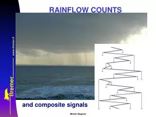
RAINFLOW COUNTS
RAINFLOW COUNTS. and composite signals. RAINFLOW COUNTS. +. +. The purpose of rainflow counting: consider a range with a wiggle on the way, it can be split into two half-cycles in several ways. Not that interesting. MUCH BETTER !. RAINFLOW COUNTS. Rainflow counting:

RAINFLOW COUNTS
E N D
Presentation Transcript
RAINFLOW COUNTS and composite signals Michel Olagnon
RAINFLOW COUNTS + + The purpose of rainflow counting: consider a range with a wiggle on the way, it can be split into two half-cycles in several ways. Not that interesting MUCH BETTER ! Michel Olagnon
RAINFLOW COUNTS Rainflow counting: Let not small oscillations (small cycles) stop the “flow” of large amplitude ones. Rainflow was originally defined by T. Endo as an algorithm (1968, 1974), another equivalent algorithm (de Jonge, 1980), that is easier to implement, is generally recommended (ASTM,1985), and a pure mathematical definition was first found by I. Rychlik (1987). Michel Olagnon
RAINFLOW COUNTS • The Endo algorithm: • turn the signal around 90° • make water flow from its upper corner on each of the “pagoda roofs” so defined, until either a roof on the other side extends opposite beyond the starting point location, or the flow reaches a point that is already wet. • Each time, a half-cycle is so defined, and most of them can be paired into full cycles (all could be if the signal was infinite). Michel Olagnon
RAINFLOW COUNTS • The ASTM algorithm: for any set of 4 consecutive turning points, • Compute the 3 corresponding ranges (absolute values) • If the middle range is smaller than the two other ones, extract a cycle of that range from the signal and proceed with the new signal • The remaining ranges when no more cycle can be extracted give a few additional half cycles. Michel Olagnon
RAINFLOW COUNTS The same ASTM algorithm is sometimes also called “rainfill”. Michel Olagnon
RAINFLOW COUNTS The mathematical definition: Consider a local maximum M. The corresponding minimum in the extracted rainflow count of cycles is max(L, R) where L and R are the overall minima on the intervals to the left and to the right until the signal reaches once again the level of M. Michel Olagnon
RAINFLOW COUNTS Rainflow is a nice way to separate small, uninteresting oscillations from the large ones, without affecting turning points by the smoothing effect of a filter nor interrupting a large range before it is actually completed. Especially, in fatigue damage calculations, small amplitude ranges can often be neglected because they do not cause the cracks to grow. Michel Olagnon
RAINFLOW COUNTS The mathematical definition allows, for discrete levels, to calculate the rainflow transition matrix from the min-max transition matrix of a Markov process. Thus, for instance, if the min-max only were recorded on a past experiment, a rainflow count can still be computed. Michel Olagnon
RAINFLOW COUNTS When dealing with stationary Gaussian processes, a number of theoretical results are available that enable in most cases to compute the rainflow count (and the corresponding fatigue damage) exactly though not always quickly. The turning points normalized by have distribution sqrt(1-2)R+ N where N is a normalized normal distribution, R a normalized Rayleigh distribution, is the standard deviation of the signal and is the spectral bandwidth parameter. When the narrow-band approximation can be used (=0), and damage is of the Miner form (D=iim, where i is the number of cycles of range i), damage can be computed in closed-form since the moments of the Rayleigh distribution are related to the function and ranges can be taken as twice the amplitude of maxima. Michel Olagnon
RAINFLOW COUNTS • When the narrow-band approximation cannot be used, the following results apply: • The narrow-band approximation provides conservative estimates of the actual rainflow damage. • If a power spectral density is given for the signal, the rainflow transition probabilities and range densities can be computed exactly, and thus also the fatigue damage. • If the original process is not gaussian, the use of an appropriate transformation to bring its probability density to the normal distribution is generally sufficient to have the gaussian process results apply to the transformed process (though “gaussian process” implies more than just normal probability density for the signal). Michel Olagnon
RAINFLOW COUNTS If a power spectral density is given for the signal, the rainflow transition probabilities and range densities can be computed exactly,.. Why that ? The interesting joint probability is p(x, x’, x” | x0, x’0, x”0). It allows to find the probability distribution for the trough associated to a given peak level in the signal. For a gaussian process, all those distributions are multidimensional gaussian ones. The spectrum is FT(E(x(t- )x(t))), it gives all the correlation functions implying the signal and its derivatives. Michel Olagnon
RAINFLOW COUNTS West Africa Spectra -> Composite signals Michel Olagnon
RAINFLOW COUNTS Some ideas about how to deal with composite signals: Michel Olagnon
RAINFLOW COUNTS Separate the turning points into two sets: * The maximum (and resp. minimum) over each interval where the low frequency signal is positive (resp. negative) * The other turning points Michel Olagnon
RAINFLOW COUNTS • The other turning points: • Their number is clearly (NH-NL) • The average rainflow damage per cycle of the high frequency signal is conservative with respect to that of those remaining turning points. • Proof: Cycles belonging to a (ML,mL) interval are mainly of the form (mH,MH) and their amplitude is thus reduced by the underlying low-frequency. Similarly for cycles belonging to a (mL,ML) interval, of the form (MH, mH). • CONSERVATIVE DAMAGE ESTIMATE: (NH-NL)/NH DH Michel Olagnon
RAINFLOW COUNTS The maximum (and resp. minimum) over each interval where the low frequency signal is positive (resp. negative) Estimates of the corresponding damage can use the narrow-band approximation. The DNV formula by Lotsberg (2005) uses a sum of sine waves approach, and thus D=NL((DH/NH)1/m + (DL/NL)1/m)m or it says that the red turning points are Rayleigh distributed with the parameter of the distribution being the sum of the two parameters for high- and low- frequency. In fact, the red process is extracted from the global gaussian process, the turning points’ probability density of which is given by the Rayleigh*Gaussian formula, and thus a damage approximation is D=NL/K(2sqrt(2M0))m E((ML/sqrt(M0))m) where the expectancy is computed using whatever knowledge of the distribution of Ml we can make out. Michel Olagnon
RAINFLOW COUNTS The SS formula D = DH + DL The CS formula D = NH+L((DH/NH)2/m + (DL/NL)2/m)m/2 The DNB formula D = (NH-NL)/NH DH + NL((DH/NH)1/m + (DL/NL)1/m)m The new formulae D = (NH-NL)/NH DH + F(L/H+L ,NL/NH, m) DL The exact formula D = WAFO (Combined Spectrum) Michel Olagnon
RAINFLOW COUNTS • The new formulae D = (NH-NL)/NH DH + F(, , m) DL • ML distributed as the maximum of NH/Nl maxima of the global signal : D = (1-)DH + Z1(m, ) ((1-2)/(1-2))m/2 DL • ML distributed as the highest NH/Nl maxima of the global signal :D = (1-)DH + Z2(m, ) ((1-2)/(1-2))m/2 DL • ML distributed as the highest NH/Nl narrow-band maxima of the global signal :D = (1-)DH + 1/ Q(m/2+1, -Ln()) / (1-2)m/2 DL • DDNB = (1-)DH + (1+ /(1-2))m DL Michel Olagnon
RAINFLOW COUNTS A few topics: A. How conservative is the narrow-band approximation for a unimodal spectrum ? B. How good are MC simulations wrt exact WAFO calculations ? C. How good are the various formulas ? D. What is a “conservative climate” ? Michel Olagnon
RAINFLOW COUNTS • A. How conservative is the narrow-band approximation for a unimodal spectrum ? • It may be noted that M0 and M2 are normalizing factors, and thus normalized damage for a Pierson-Moskowitz depends only on m, for a Jonswap on m and , etc. • Sensitivityto spectral bandwidth. • Sensitivity to spectral shape. • Sensitivity to cut-off frequency. Michel Olagnon
RAINFLOW COUNTS • B. How good are MC simulations wrt exact WAFO calculations ? • Sensitivity to the number of simulations. • Sensitivity to alea modeling (random phases/complex spectrum). • Sensitivity to stationarity (high- or low-frequency consisting of impulse-like responses from time to time). Michel Olagnon
RAINFLOW COUNTS • C. How good are the various formulas ? • vs. , the normalized low-frequency standard-deviation • vs. , the normalized low-frequency number of cycles • vs. the bandwidth of the high-frequency signal. Michel Olagnon
RAINFLOW COUNTS D. What is a “conservative climate” ? How to sample the parameter space so as to keep number of structural computation cases low and still have good damage estimates ? Can we use average values of the F(, , m) functions, or even of , to directly sum separately the low and high frequency damages in some regions of the parameter space ? Michel Olagnon
RAINFLOW COUNTS Sensitivityto spectral bandwidth. Michel Olagnon
RAINFLOW COUNTS Sensitivityto spectral bandwidth. Michel Olagnon
RAINFLOW COUNTS Sensitivityto amplitude filtering. Michel Olagnon
RAINFLOW COUNTS Sensitivity tocut-off frequency. (without M0 correction) Michel Olagnon
RAINFLOW COUNTS Sensitivitytocut-off frequency. (with M0 correction) Michel Olagnon
RAINFLOW COUNTS Sensitivitytocut-off frequency. A simple way to find a reasonable cut-off frequency for waves : For amplitudes less than 0.2 HS, we see no change in the damage when filtering them out. Assuming a global steepness of the sea state of 6% (wind sea), waves of 0.2 HS break for periods smaller than TZ/ 3.5. It is thus reasonable to cut the spectrum at about 4 fp of the wind sea. In the case of a Pierson-Moskowitz spectrum, the resulting is 0.66, i.e. same as for white noise. Michel Olagnon
RAINFLOW COUNTS Sensitivity to the number/length of simulations. Michel Olagnon
RAINFLOW COUNTS Sensitivity to the number/length of simulations. Michel Olagnon
RAINFLOW COUNTS • The new formulae D = (NH-NL)/NH DH + F(, , m) DL • ML distributed as the maximum of NH/Nl maxima of the global signal : D = (1-)DH + Z1(m, ) ((1-2)/(1-2))m/2 DL • ML distributed as the highest NH/Nl maxima of the global signal :D = (1-)DH + Z2(m, ) ((1-2)/(1-2))m/2 DL • ML distributed as the highest NH/Nl narrow-band maxima of the global signal :D = (1-)DH + Q(m/2+1, -Ln()) / (1-2)m/2 DL • DDNB = (1-)DH + (1+ /(1-2))m DL Michel Olagnon
RAINFLOW COUNTS Dependence of coefficient to DL vs. Michel Olagnon
RAINFLOW COUNTS 1 m swell, 14s + 2 m wind sea, 7s Michel Olagnon
RAINFLOW COUNTS 1 m swell, 14s + 2 m wind sea, 7s + 4 m, 140 s Michel Olagnon