Download
1 / 55
570 likes | 776 Vues
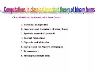
1. . Historical Bac. k. gro. u. nd. 2. I. n. var. i. ants. a. nd. C. o. v. ariants of binar. y forms. 3. Sym. b. olic. metho. d. of. Ar. o. n. h. o. l. d. 4. Bracket . P. o. l. ynom. i. als. 5. D. i. graphs a. n. d. M. olecules. 6. Syzygies an. d.

E N D
1 . Historical Bac k gro u nd 2. I n var i ants a nd C o v ariants of binar y forms 3. Sym b olic metho d of Ar o n h o l d 4. Bracket P o l ynom i als 5. D i graphs a n d M olecules 6. Syzygies an d the Algeb r a o f Digraphs 7. Tr a nsv ectants 8. Finding the Hilbert basis Computations in classical invariant theory of binary forms Cheri Shakiban (Joint work with Peter Olver)
Interesting note: Cayley won the first Smith prize at Cambridge. Quiz: How many mathematical papers did he publish? 1. Historical background 19th- Century George Boole (1815-1864) He was one of the first to notice that invariants were important. Interesting note: Boole’s daughter Alicia Boole Stott (1860-1949) was a mathematician. Arthur Cayley (1821-1895) Cayley was aware of invariants up to degree 6 but thought binary forms of degree 7 or more didn’t have a basis for their Invariants.
Paul Albert Gordan(1837 – 1912) In 1868, Gordan gave a constructive proof that the covariants and invariants of a binary form of any degree has a finite basis. , • Quiz:Who was Gordan’s only student? James Sylvester (1814-1897) Quiz: Who was Sylvester’s most famous student? What famous journal did he start?
Sylvester produced tables for the bases of the invariants and covariants: Degree 2 3 4 5 6 7 8 9 10 12 # Invariants 1 1 2 4 5 26(30) 9 89 104 109 # Covariants 2 4 5 23 26 124(130) 69 415 475 949 Degree 8: The invariants/covariants were checked by Shioda in 1967 Degree 7: Constructed by Dixmier in 1992. New proof: Leonid Bedratyuk Feb 2006 http://front.math.ucdavis.edu/math.AG/0602373 http://front.math.ucdavis.edu/math.AG/0611122 Courtesy of Alicia Dickenstein Classical Invariant Theory by Peter J. Olver
Death-blow: Hilbert's celebrated Basis Theorem. Any finite system of homogeneous polynomials admits a finite basis for its invariants, as well as for its covariants (1888). David Hilbert (1862-1943) The first proof was existential. Gordan’s comment: Das ist Theologie und nicht Mathematick Hilbert published a second constructive proof. Hilbert was unjustly saddled with the reputation of killing off constructive invariant theory. It was really a slow death. As pointed out by Bernd Sturmfels: Hilbert’s second proof combined with the theory of Gröbner bases can be used to construct an algorithm producing the Hilbert bases of a general system of forms.
Graphical Methods: William Clifford (1845-1879) Clifford: began developing a graphical method for the description of the invariants and covariants of binary forms. Sylverster: unveiled his “ algebro-chemical theory”, whose aim was to apply the methods of classical invariant theory to the rapidly developing science of molecular chemistry.
Recent years: interest in classical invariant theory is on the rise. Dynamical systems Solution of nonconvex variational problems Elasticity Molecular physics Modular forms Computer vision Others • Revival of the computational approach: partly due to • current availability of symbolic manipulation computer • programs.
where is nonsingular The polynomial is given by
Definitions: A n in v arian t o f weight g of a b i nary A covarian t of we i gh t g is a f u n c tio n J( a , x ) form Q( x ,y) , o f degree n, is a f unct i on
The most important covariantof a quartic, or, indeed, of any binary form Q is the Hessian degree 2n – 4, covariant of weight 2. Besides Q itself , there is only one other independent covariant of the quartic: Jacobian of Q and H.
Siegfried Aronhold(1819 - 1884) The first German to work in this topic. The motivating idea: We can pretend that abinary form Q(x,y) is just the nth power of a linear form is a “symbolic letter”
To resolve this ambiguity , we use a different symbolic letter for each occurrence of coefficients ai:
and so on.
There is a unique symmetric symbolic form for any given polynomial, obtained by symmetrizing any given representative over all the symbolic letters occurring in it. has symmetric symbolic form
Theorem: Each polynomial has a unique symmetric symbolic form The number of different symbolic letters in a symbolic polynomial represents the degree of the polynomial in the coefficients of the form. Example: The invariant of the binary quartic,
Again, we see a similar factorization as with the discriminant of the binary quadratic. Example of a covariant: The Hessian of the quartic Symbolic covariant
Bracket Polynomials. Definition: a) A bracket factor of the first kind is a linear monomial b) A bracket factor of the second kind is where are distinct symbolic letters.
The First Fundamental Theorem of Invariant Theory states that every covariant of a binary form can be written in symbolic form as a bracket polynomial. The degree of the covariant in the coefficients ai is equal to the number of distinct symbolic letters occurring in the bracket polynomial representative. The weight of the covariant is equal to the number of bracket factors of the second kind in any monomial of P. The degree of the covariant in the variables x is equal to the number of bracket factors of the first kind in any monomial of P.
Example: In the case of a quartic form, The invariants Similarly: The Hessian The other covariant
The symbolic form of a given covariant does not have a unique bracket polynomial representative, owing to the presence of certain syzygies among the bracket factors themselves. There are three of these fundamental syzygies: [a b] = – [b a] . [a b] (g x) = [a g] (b x) + [g b] (a x). 3. [a b] [g d] = [a g] [b d] + [a d] [g b]. Here are distinct symbolic letters.
Remark on bracket polynomials: If we know the degree of a covariant, and just the bracket factors of the second kind in any homogeneous bracket polynomial representative, we can reconstruct the bracket factors of the first kind. Example: If we have a symbolic monomial of degree 3 in the coefficients ai of the form whose bracket factors of the second kind are [a b] [b g]2
The full bracket monomial must be 2 ( x)n–1 ( x)n–3 (x)n–2, n = degree since occurs once, three times, and twice in the second factors. If the degree of the covariant is 4 2 ( x)n–1 ( x)n–3 ( x)n–2 ( x)n. We can concentrate on the bracket factors of the second kind and drop ( x)n–1 ( x)n–3 ( x)n–2 ( x)n…. We will call them just brackets for short.
5.Digraphs and Molecules Graphical method: Consider a binary form of degree n, and let P be a bracket polynomial representing the symbolic form of some covariant. To each monomial in P we will associate a "molecule", or, more mathematically, a digraph. Algebro-chemical theory as proposed by Sylvester: Let M be any unit bracket monomial (with coefficient 1). To each distinct symbolic letter in M we associate an atom. For a binary form of degree n, the atoms will all have "valence" n.
Example: Consider the Hessian of a binary form of degree n. It has the symbolic form 2 ( x)n–2 ( x)n–2. Molecule will consist of two atoms. Since the bracket factor occurs twice, there will be two directed bonds from atom to atom . Thus the directed molecule representing the Hessian is
The discriminant of the binary cubic, has symbolic bracket expression It is represented by the neutral four-atom molecule
* The bonds in our molecule will correspond to all the bracket factors of the second kind occurring in M. * If is a bracket in M, then we have a bond between the atom labeled and the atom labeled . * If a bracket occurs to the kth power - k - in M, then there will be k bonds between atom and atom . The key: To make use of directed (or polarized) bonds, which will enable us to distinguish between the bracket factors and . = –
The molecular representation does not depend on how we label the constituent atoms. can represented by any of the equivalent forms etc. We can drop the labels for the individual atoms, and concentrate on the pure "chemistry" of our molecule. is the molecular representation of the Hessian. is the molecular representation of the discriminant of the binary cubic.
Representation of covariants Ions: If there are one or more atoms with unused free bonding sites, the valence is strictly positive and we say we have an ion. Neutral molecules : If an atom has exactly n bonds, and the entire molecule has valence 0. Neutral molecules correspond to invariants, while ions correspond to more general covariants. saturated digraph n=4 covariant n=3 invariant x) x) x) x) irreducible reducible Note: we must have exactly n of each symbols.
Linear combination of molecules: Example: In the case of a binary cubic, the bracket monomial M1 = 2 x) (x)2 has molecular representation n=3 D1 = while M2 = x) xx) has molecular representation D2 =
Therefore, the bracket polynomial P = 2 x)(x)2 – 1/2xx)(x) has molecular representation 2D1 – 1/2 D2 = 2 – 1/2 Chemical analogy: These linear combinations of molecules might be interpreted as "mixtures" of molecular substances, although the admission of negative coefficients stretches this analogy rather thin.
Mathematically: What we are doing is replacing each unit bracket monomial by a digraph. Recall that a graph is: a collection of vertices and line segments connecting the vertices. A digraph is: a graph in which the line segments are arrows. D1 D2 D3 represent distinct digraphs.
Note that the digraph , the mirror image of D2, is really the same as D2: Any bracket monomial will have a unique digraph representation. In a digraph, the vertices correspond to the atoms in the molecular representation, and the darts correspond to the directed bonds.
Theorem . Let Q be a binary form of degree n. Then there is a one-to-one correspondence between bracket polynomials representing covariants of Q and elements of the space Dn of linear combinations of n-digraphs. A digraph is reducible if it is the disjoint union of two subdigraphs. Example: The reducible digraph on four vertices represents the square of the Hessian H of a form: H2.
6. Syzygies and the Algebra of Digraphs There are three basic rules in the algebra of digraphs: Rule #1. From the first syzygy – , = – Applications of rule #1: a) Dropping the inessential symbolic labels for the vertices, implies = — 2 = 0 Hence represents the trivial covariant 0.
b) Consider the bracket monomial x)n–2 ( x)n–2 ( x)n–2. However, this monomial is a symbolic form of the trivial (zero) covariant. (Verify algebraically!). Graphically: If we reverse the direction of all three darts in the digraph, we see that 3 = (–1) = – 2 = 0 is equivalent to the trivial digraph.
= + Rule #2. The syzygy x x) + x), translates into the digraph rule
= + = + = – – Applications of rule #2 a) Consider the digraph By Rule #1, we find But all three of these digraphs are exactly the same, hence = 0 3
= + Rule #3. The remaining syzygy has the form
D = We can denote double bonds which point in the same direction by plain line segments, so Is equivalent to Applications of rule #3: we can show that the digraph or corresponding to the bracket monomial x)n–2 x)n–3 x)n–2 x)n–2 x)n–1 is equivalent to a reducible digraph. so this bracket monomial corresponds to a covariant which is the product of two simpler covariants.
= + – =– Apply Rule #1 to the bottom dart, D =– Apply Rule #3 to the top and bottom darts,
R = On the right hand side, the first digraph is reducible. Untangling the second digraph, and reversing the directions of two darts, we get D = – R – D, where R is reducible, hence D = – 1/2 R is also reducible.
7. Transvectants. Given a molecular ion representing a covariant of a binary form, we can obtain new, more complicated molecules by "reacting" with other ions, in particular with free atoms. The invariant theoretic name for this reaction is transvection, and it provides a ready mechanism for constructing new covariants from old ones. Example: Consider the digraph T = which represents the covariant T of the binary quartic.
The first transvectant (Q,T)(1). This will be a linear combination of all possible digraphs which can be obtained by joining a single atom or vertex, representing the quartic Q itself, to the digraph for T with a single dart. There are three possible such digraphs: D1 = D2 = 2 free bonds in D1 D3 = 1 free bond in D2 Therefore (Q,T)(1) = 2D1 + D2 + 3D3. 3 free bonds in D3
The second transvectant (Q,T)(2): It will be a linear combination of all possible digraphs which can be obtained by joining a single atom by two darts to the digraph for T. There are five possible such digraphs: D1 = D2 = D3 = D4 = D5 = (Q,T)(2) = 2D1 + 4D2 + 12D3 + 6D4 + 3D5.
Finding the Hilbert basis Gordan’s method for constructing a Hilbert basis for the covariants of binary forms: Start with the form Q itself. Use successive transvectants with Q to recursively construct covariants of the next higher degree (using certain rules). 3. Use the syzygies to eliminate redundant covariants. 4. Stop when you don’t get anything new. Gordan proved that this algorithm terminates (1868). Note: You only need to consider one digraph in each transvectant.
Quadratic case: For a quadratic, we are working in the space of 2-digraphs, so we can attach at most 2 darts to any given vertex. We begin with the form Q itself. There are only two possible transvectants: and The first is trivial by Rule #1, and the second is the Hessian which is an invariant. we cannot get anything further by transvecting again. We are done. That the only covariants of a binary quadratic are the form itself and its discriminant.
Cubic case :Turning to the binary cubic, we begin with Q 1 from which we can form three transvectants: Trivial by Rule #1 Trivial by Rule #1 2 H So we can form the two further transvectants: 3 Trivial by Rule #2