Download
1 / 32
330 likes | 646 Vues
Linear Systems of Equations. Direct Methods for Solving Linear Systems of Equations. for unknown. are known for. Operations to simplify the linear system ( . is constant):. Direct Methods for Solving Linear Systems of Equations. The linear system.

E N D
for unknown are known for Operations to simplify the linear system ( is constant): Direct Methods for Solving Linear Systems of Equations The linear system
The system is now in triangular form and can be solved by a backward substitution process Direct Methods Example:
Definitions An nxm (n by m) matrix: The 1xn matrix (an n-dimensional row vector): The nx1 matrix (an n-dimensional column vector):
Definitions then is the augmented matrix.
with Gaussian Elimination with Backward Substitution The general Gaussian elimination applied to the linear system First form the augmented matrix
provided , yields the resulting matrix of the form Gaussian Elimination with Backward Substitution The procedure which is triangular.
when Gaussian Elimination (cont.) Since the new linear system is triangular, backward substitution can be performed
Gaussian eliminations requires arithmetic operations. Cramer’s rule requires about arithmetic operations. A simple problem with grid 11 x 11 involves n=81 unknowns, which needs operations. years ! About Gaussian Elimination and Cramer’s Rule What time is required to solve this problem by Cramer’s rule using 100 megaflops machine?
A diagonal matrix is a square matrix with whenever An upper-triangular nxn matrix has the entries: A lower-triangular nxn matrix has the entries: More Definitions The identity matrix of order n, is a diagonal matrix with entries
Do you see that ? Do you see that A can be decomposed as: Examples ?
Matrix Form for the Linear System The linear system can be viewed as the matrix equation
because we can rewrite the matrix equation Solving by forward substitution for y and then for x by backward substitution, we solve the system. LU decomposition The factorization is particularly useful when it has the form
Matrix Factorization: LU decomposition Theorem: If Gaussian elimination can be performed without row interchanges, then the decomposition A=LU is possible, where
An iterative technique to solve Ax=b starts with an initial approximation and generates a sequence First we convert the system Ax=b into an equivalent form The stopping criterion: Iterative Methods And generate the sequence of approximation by This procedure is similar to the fixed point method.
Iterative Methods (Example) We rewrite the system in the x=Tx+c form
and start iterations with Iterative Methods (Example) – cont. Continuing the iterations, the results are in the Table:
The JacobiIterative Method The method of the Example is called the Jacobi iterative method
The JacobiMethod: x=Tx+c Form (cont) and the equation Ax=b can be transformed into Finally
The idea of GS is to compute using most recently calculated values. In our example: Starting iterations with , we obtain The Gauss-SeidelIterative Method
Gauss-Seidel in form (the Fixed Point) The Gauss-SeidelIterative Method Finally
The SOR is devised by applying extrapolation to the GS metod. The extrapolation tales the form of a weighted average between the previous iterate and the computed GS iterate successively for each component where denotes a GS iterate and ω is the extrapolation factor. The idea is to choose a value of ωthat will accelerate the rate of convergence. under-relaxation over-relaxation The Successive Over-Relaxation Method (SOR)
SOR: Example Solution: x=(3, 4, -5)