Advanced Nonlinear Programming Methods
Explore the complexity and challenges of nonlinear programming compared to linear programming, covering optimization techniques and conditions for finding optimal solutions. Includes classical optimization, necessary conditions for local and global minima, and convexity properties.


Advanced Nonlinear Programming Methods
E N D
Presentation Transcript
Chapter 10 Nonlinear Programming Methods
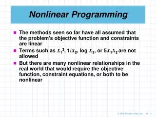
Background • Solution techniques for nonlinear programming (NLP) are much more complex and much less effective than those for linear programming (LP). • Linear programming codes will provide optimal solutions for problems with hundreds of thousands of variables, but there is a reasonable chance that an NLP code will fail on a problem containing only a handful of variables. • To sharpen this contrast, recall that all interior point methods for solving LP problems include ideas originally developed to solve NLP problems.
10.1 CLASSICAL OPTIMIZATION The simplest situation that we address concerns the minimization of a function f in the absence of any constraints. This problem can be written as Minimize {f(x):x Rn} Where f C2 (twice continuously differentiable). Without additional assumptions on the nature of f, we will most likely have to be content with finding a point that is a local minimum. Elementary calculus provides a necessary condition that must be true for an optimal solution of a nonlinear function with continuous first and second derivatives. • gradient is zero at every stationary point that is a candidate for a maximum or minimum. • Sufficient conditions derived from convexity properties are also available in many cases.
Unconstrained Optimization The first-order necessary condition that any pointx* must satisfy to be a minimum of f is that the gradient must vanish. ▽f(x*)=0 (2) This property is most easily illustrated for a univariate objective function in which the gradient is simply the derivative or the slope of f(x). Consider, for example, Figure 10.1. The function in part (a) has a unique global minimum x* at which the slope is zero. Any movement from that point yields a greater, and therefore less favorable, value. The graph in part (b) exhibits a range of contiguous global minima where the necessary condition holds; however, we should note that the corresponding f(x) is not twice continuously differentiable at all points.
Figure 10.2 shows why Equation (2) is only a necessary condition and not a sufficient condition. In all three parts of the figure there are points at which the slope of f(x) is zero but the global minima are not attained. Figure 10.2a illustrates a strong local maximum at x1*and a strong local minimum at x2*. Figure 10.2b shows a point of inflection at x1* that is a one-dimensional saddle point. Finally, Figure 10.2c presents the case of a unique global maximum at x1*. The ideas embodied in Figures 10.1 and 10.2 can be easily generalized to functions in a higher-dimensional space at both the conceptual and mathematical levels. Because the necessary condition that the gradient be zero ensures only a stationary point—ie., a local minimum, a local maximum, or a saddle point at x*.
Sufficient conditions for x* to be either a local or a global minimum: • If f(x) is strictly convex in the neighborhood of x*, then x* is a strong local minimum. • If f(x) is convex for all x, then x* is a global minimum. • If f(x) is strictly convex for all x, then x* is a unique global minimum. To be precise, a neighborhood of x is an open sphere centered at x with arbitrarily small radius ε > 0. It is denoted by Nε(x), where Nε(x) = {y : ∥ (y - x) ∥ < ε}.
f(x) is strictly convex if its Hessian matrix H(x) is positive definite for all x. In this case, a stationary point must be a unique global minimum. f(x) is convex if its Hessian matrix H(x) is positive semidefinite for all x. For this case a stationary point will be a global (but perhaps not unique) minimum. If we do not know the Hessian for all x, but we evaluate H(x*) at a stationary point x* and find it to be positive definite, the stationary point is a strong local minimum. (If H(x*) is only positive semidefinite at x* , x* can not be guaranteed to be a local minimum.)
Functions of a Single Variable Let f(x) be a convex function of x . A necessary and sufficient condition for x* to be a global minimum is that the first derivative of f(x) be zero at that point.This is also a necessary and sufficient condition for the maximum of a concave function. The optimal solution is determined by setting the derivative equal to zero and solving the corresponding equation for x. If no solution exists, there is no finite optimal solution. A sufficient condition for a local minimum (maximum) point of an arbitrary function is that the first derivative of the function be zero and the second derivative be positive (negative) at the point.
Example 1 Let us find the minimum of f(x) = 4x2 - 20x + 10. The first step is to take the derivative of f(x) and set it equal to zero. d f(x)/dx=8x-20=0 Solving this equation yields x* = 2.5 , which is a candidate solution. Looking at the second derivative, we see d2 f(x)/dx2=8>O for all x so f is strictly convex. Therefore, x* is a global minimum.
Example 2 As a variation of Example 1, let us find the minimum of f(x) = -4x2 - 20x. Taking the first derivative and setting it equal to zero yields df(x)/dx = -8x - 20 = 0, so x* = -2.5. The second derivative is d2f(x)/dx = -8 < 0 for all x, so f is strictly concave. This means that x* is a global maximum. There is no minimum solution because f(x) is unbounded from below.
Example 3 Now let us minimize the cubic function f(x) = 8x3 + 15x2 + 9x + 6. Taking the first derivative and setting it equal to zero yields df(x)/dx = 24 x2 + 30x + 9 = (6x + 3)(4x + 3) = 0. The roots of this quadratic are at x = -0.5 and x = -0.75, so we have two candidates. Checking the second derivative d2f(x)/dx2 = 48x + 30 we see that it can be > 0 or < 0. Therefore,f(x) is neither convex nor concave. At x = -0.5, d2f(-0.5)/dx2 = 6, so we have a local minimum. At x = -0.75, d2f(-0.75)/dx2 = -6, which indicates a local maximum. These points are not global optima, because the function is actually unbounded from both above and below.
Functions of Several Variables Theorem 1: Let f(x) be twice continuously differentiable throughout a neighborhood of x*. Necessary conditions for x* to be a local minimum of f are a.▽f(x*)=0 b.H(x*) is positive semidefinite.
Theorem 2: Let f(x) be twice continuously differentiable throughout a neighborhood of x*. Then a sufficient condition for f(x) to have a strong local minimum at x*, where Equation (2) holds, is that H(x*) be positive definite. Note: H(x*) being positive semidefinite is not a sufficient condition for f(x) to have a local minimum at x*.
Quadratic Forms A common and useful nonlinear function is the quadratic function that has coefficients a , c, and Q . Q is the Hessian matrix of f(x). Setting the gradient ▽ to zero results in a set of n linear equations in n variables. A solution will exist whenever Q is nonsingular. In such instances, the stationary point is x*= -Q-1cT
For a two-dimensional problem, the quadratic function is For this function, setting the partial derivatives with respect to x1, and x2 equal to zero results in the following linear system.
These equations can be solved using Cramer's rule from linear algebra. The first step is to find the determinant of the Q matrix. Let The appropriate substitutions yield which is the desired stationary point.
When the objective function is a quadratic, the determination of definiteness is greatly facilitated because the Hessian matrix is constant. For more general forms, it may not be possible to determine conclusively whether the function is positive definite, negative definite, or indefinite. In such cases, we can only make statements about local optimality. In the following examples, we use H to identify the Hessian. For quadratic functions, Q and H are the same.
Example 4 Find the local extreme values of Solution: Using Equation (2) yields 50 X1 - 20 = 0 and 8 X2 + 4 = 0 The corresponding stationary point isx* = (2/5, -1/2). Because f(x) is a quadratic, its Hessian matrix is constant. The determinants of the leading submatrices of H are H1 = 50 and H2 = 400, so f(x) is strictly convex, implying that x* is the global minimum.
Example 5 Find the local extreme values of the nonquadratic function Solution: Using Equation (2) yields ▽f(x)=(9x12 –9, 2x2 +4) T =(0, 0) T So x1 = ±1 and x2= -2. Checking x = (1, -2), we have
which is positive definite since vT H(l, -2)v =18 v12 + 2v22 > 0 when v≠0. Thus (1, -2) yields a strong local minimum. Next, consider x = (-1, -2) with Hessian matrix Now we have vT H(-l, -2)v =-18 v12 + 2v22, which may be less than or equal to 0 when v≠0. Thus, the sufficient condition for (-1, -2) to be either a local minimum or a local maximum is not satisfied. Actually, the second necessary condition (b) in Theorem 1 for either a local minimum or a local maximum is not satisfied. Therefore, x = (1, -2) yields the only local extreme value of f.
Example 6 Find the extreme values of f(x) = -2x12+ 4x1 x2-4x22 + 4x1 + 4x2 +10. Solution: Setting the partial derivatives equal to zero leads to the linear system -4 x1 + 4 x2+ 4 = 0 and 4 x1 -8 x2+ 4 = 0 which yields x* = (3, 2). The Hessian matrix is Evaluating the leading principal determinants of H, we find H1= -4 and H2 = 16. Thus, f(x) is strictly concave andx* is a global maximum.
Nonquadratic Forms When the objective function is not quadratic (or linear), the Hessian matrix will depend on the values of the decision variables x. Suppose The gradient of this function is
For the second component of the gradient to be zero , we must have x2= . Taking this into account, the first component is zero only when x1= 1, so x* = (1,1) is the sole stationary point. It was previously shown (in Section 9.3) that the Hessian matrix H(x) at this point is positive definite, indicating that it is a local minimum. Because we have not shown that the function is everywhere convex, further arguments are necessary to characterize the point as a global minimum. Logically, f(x)≧0 because each of its two component terms is squared. The fact that f(1,1) = 0 implies that (1,1) is a global minimum. As a further example, consider
where A stationary point exists at x* = (0, 0). Also, H1 = 2 and H2 = 44x22 - 20x1 implying that H(x) is indefinite. Although H(x) is positive semidefinite at (0,0) this does not allow us to conclude that x* is a local minimum. Notice that f(x) can be made arbitrarily small or large with the appropriate choices of x. These last two examples suggest that for nonquadratic functions of several variables, the determination of the character of a stationary point can be difficult even when the Hessian matrix is semidefinite. Indeed, a much more complex mathematical theory is required for the general case.
Summary for Unconstrained Optimization Table 10.1 summarizes the relationship between the optimality of a stationary point x* and the character of the Hessian evaluated at x*. It is assumed that f(x) is twice differentiable and ▽f(x*) = 0. If H(x) exhibits either of the first two definiteness properties for all x, then "local" can be replaced with "global" in the associated characterizations. Furthermore, if f(x) is quadratic, a positive semidefinite Hessian matrix implies a nonunique global minimum at x*.
Notice that although convexity in the neighborhood of x* is sufficient to conclude that x* is a weak local minimum, the fact that H(x*) is positive semidefinite is not sufficient, in general, to conclude that f(x) is convex in the neighborhood of x*.
When H(x*) is positive semidefinite, it is possible that points in a small neighborhood of x* can exist such that f(x) evaluated at those points will produce smaller values than f(x*). This would invalidate the conclusion of convexity in the neighborhood of x*. As a final example in this section, consider for which
and Looking at the Hessian matrix, it is virtually impossible to make any statements about the convexity of f(x).This gives us a glimpse of the difficulties that can arise when one attempts to solve unconstrained nonlinear optimization problems by directly applying the classical theory. In fact, the real value of the theory is that it offers insights into the development of more practical solution approaches. Moreover, once we have a stationary point x* obtained from one of those approaches, it is relatively easy to check the properties of H(x*), because only numerical evaluations are required.
A Taylor series is a series expansion of a function about a point. A one-dimensional Taylor series is an expansion of a real function about a point a is given by If a=0, the expansion is known as a Maclaurin series.
Nonnegative Variables A simple extension of the unconstrained optimization problem involves the addition of non-negativity restrictions on the variables. Minimize [f(x):x≧0] (3) Suppose that f has a local minimum at x*, where x*≧0. Then there exists a neighborhood Nε(x*) of x* such that whenever x Nε(x*) and x > 0, we have f(x) ≧ f(x*). Now write x = x* + td, where d is a direction vector and t > 0. Assuming that f is twice continuously differentiable throughout Nε(x*), a second-order Taylor series expansion of f(x* + td) around x* yields
where α [0,1]. Canceling terms and dividing through by t yields As t —> 0, the inequality becomes 0 ≦▽f(x*)d, which says that f must be nondecreasing in any feasible direction d. Hence, if x* > 0, we know that ▽f(x*) = 0. With a bit more analysis, it can be shown that the following conditions are necessary for x* to be a local minimum of f(x).
These results are summarized as follows. Theorem 3: Necessary conditions for a local minimum of f in Problem (3) to occur at x* include ▽f(x*)≧0, ▽f(x*)x*=0, x*≧0 (4) where f is twice continuously differentiable throughout a neighborhood of x*.
a. b. c. d. e. f. Example 8 Minimize f(x) = subject to x1≧0, x2≧0,x3≧0 Solution: From Conditions (4), we have the following necessary conditions for a local minimum. g.
From condition (d), we see that either x2 = 0 or x1 = x2. When x2 = 0, conditions (c) and (g) imply that x1 = 0. From condition (f) then, x3 = 0. But this contradicts condition (a), x2 ≠0 and x1 = x2.
Condition (f) implies that either x3 = 0 or x1 = x3. If x3 = 0, then conditions (d), (e), and (g) imply that x1= x2 = x3 = 0. But this situation has been ruled out. Thus, x1= x2 = x3 , and from condition (b) we get x1 = 0 or x1 = 1. Since x1≠0, the only possible relative minimum of f occurs when x1= x2 =x3= 1. To characterize the solution at x* = (1, 1, 1) we evaluate the Hessian matrix. which is easily shown to be positive definite. Thus, f is strictly convex and has a strong local minimum at x*. It follows from Theorem 2 in Chapter 9 that f(x*) = 1 is a global minimum.
Necessary Conditions for Optimality Equality constraints: Minimize f(x) subject to gi(x) = 0, i = 1,..., m (5) The objective and constraint functions are assumed to be at least twice continuously differentiable. Furthermore, each of the gi(x) subsumes the constant term bi. To provide intuitive justification for the general results, consider the special case of Problem (5) with two decision variables and one constraint—i.e., Minimize f(x1, x2) subject to g(x1, x2)=0
To formulate the first-order necessary conditions, we construct the Lagrangian here λ is an unconstrained variable called the Lagrange multiplier. Our goal now is to minimize the unconstrained function . As in Section 10.1, we construct the gradient of the Lagrangian with respect to its decision variables x1 and x2 and the multiplier λ. Setting the gradient equal to zero, we obtain
(6) which represents three equations in three unknowns. Using the first two equations to eliminate λ, we have which yields a stationary point x* and λ* when solved. From Equation (6), we see that ▽f(x1 , x2)and ▽g(x1 , x2) are coplanar at this solution ,i.e., ▽f(x1 , x2)= λ▽g(x1 , x2) .
It is a simple matter to extend these results to the general case. The Lagrangian is where λ = ( ,..., ) is an m-dimensional row vector. Here, every constraint has an associated unconstrained multiplier . Setting the partial derivatives of the Lagrangian with respect to each decision variable and each multiplier equal to zero yields the following system of n + m equations. These equations represent the first-order necessary conditions for an optimum to exist at x*. (7a) (7b)
A solution to Equations (7a) and (7b) yields a stationary point (x*, λ*); however, an additional qualification must be placed on the constraints in Equation (7b) if these conditions are to be valid. The most common qualification is that the gradients of the binding constraints are linearly independent at a solution. Because Equations (7a) and (7b) are identical regardless of whether a minimum or maximum is sought, additional work is required to distinguish between the two. Indeed, it may be that some selection of the decision variables and multipliers that satisfies these conditions determines a saddle point of f(x) rather than a minimum or maximum.
Example 10 Minimize f(x) = (x1 + x2)2subject to - (x1 – 3)3 +x22= 0 The Lagrangian is Now, setting partial derivatives equal to zero gives three highly nonlinear equations in three unknowns:
The feasible region is illustrated in Figure 10.3. Notice that the two parts of the constraint corresponding to the positive and negative values of x2 form a cusp. At the endpoint (3,0), the second derivatives are not continuous, foreshadowing trouble. In fact, x = (3, 0) is the constrained global minimum, but on substitution of this point into the necessary conditions, we find that the first two equations are not satisfied. Further analysis reveals that no values of x1 , x2, and λ will satisfy all three equations. (Constraint qualification is not satisfied.)
The difficulty is that the constraint surface is not smooth, implying that the second derivatives are not everywhere continuous. Depending on the objective function, when such a situation arises the first-order necessary conditions [Equations (7a) and (7b)] may not yield a stationary point.
INEQUALITY CONSTRAINTS: The most general NLP model that we investigate is Minimize f(x) subject to where an explicit distinction is now made between the equality and inequality constraints. In the model, all functions are assumed to be twice continuously differentiable, and any RHS constants are subsumed in the corresponding functions hi(x) or gi (x). Problems with a maximization objective or ≧ constraints can easily be converted into the form of above problem. Although it is possible and sometimes convenient to treat variable bounds explicitly, we assume that they are included as a subset of the m inequalities.
Karush-Kuhn-Tucker (KKT) Necessary Conditions To derive first- and second-order optimality conditions for this problem, it is necessary to suppose that the constraints satisfy certain regularity conditions or constraint qualifications, as mentioned previously. The accompanying results are important from a theoretical point of view but less so for the purposes of designing algorithms. Consequently, we take a practical approach and simply generalize the methodology used in the developments associated with the equality constrained Problem (5).
In what follows, let h(x) = (h1(x),..., hP(x))T and g(x) = (g1(x),..., gm(x)) T. For each equality constraint we define an unrestricted multiplier, λi, i= 1,..., p, and for each inequality constraint we define a nonnegative multiplier,μi, i = 1,..., m. Let X, λ and μ be the corresponding row vectors. This leads to the Lagrangian for Problem (8). Definition 1: Let x* be a point satisfying the constraints h(x*) = 0, g(x*) ≦0 and let K be the set of indices k for which gk(x*) = 0. Then x* is said to be a regular point of these constraints if the gradient vectors ▽hj(x*) (1 ≦j≦p),▽gk (x*) (kK) are linearly independent (equality part).
Theorem 4(Karush-Kuhn-Tucker Necessary Conditions): Let x* be a local minimum for Problem (8) and suppose that x* is regular point for the constraints. Then there exists a vector and a vector μ* such that (9a) (9b) (9c) (9d) (9e)