Download
1 / 47
470 likes | 594 Vues
Learn key option valuation concepts, including Put-Call Parity, Black-Scholes Model, and strategies like Protective Put. Understand the relationships between option premiums, stock price, expiration time, and more. Explore examples, continuous compounding, risk-free rates, and European vs. American options.

E N D
24 Option Valuation
Key Concepts and Skills • Understand and be able to use Put-Call Parity • Be able to use the Black-Scholes Option Pricing Model • Understand the relationships between option premiums and stock price, time to expiration, standard deviation and the risk-free rate • Understand how the OPM can be used to evaluate corporate decisions
Chapter Outline • Put-Call Parity • The Black-Scholes Option Pricing Model • More on Black-Scholes • Valuation of Equity and Debt in a Leveraged Firm • Options and Corporate Decisions: Some Applications
Protective Put • Buy the underlying asset and a put option to protect against a decline in the value of the underlying asset • Pay the put premium to limit the downside risk • Similar to paying an insurance premium to protect against potential loss • Trade-off between the amount of protection and the price that you pay for the option
An Alternative Strategy • You could buy a call option and invest the present value of the exercise price in a risk-free asset • If the value of the asset increases, you can buy it using the call option and your investment • If the value of the asset decreases, you let your option expire and you still have your investment in the risk-free asset
Comparing the Strategies • Stock + Put • If S < E, exercise put and receive E • If S ≥ E, let put expire and have S • Call + PV(E) • PV(E) will be worth E at expiration of the option • If S < E, let call expire and have investment, E • If S ≥ E, exercise call using the investment and have S
Put-Call Parity • If the two positions are worth the same at the end, they must cost the same at the beginning • This leads to the put-call parity condition • S + P = C + PV(E) • If this condition does not hold, there is an arbitrage opportunity • Buy the “low” side and sell the “high” side • You can also use this condition to find the value of any of the variables, given the other three
Example: Finding the Call Price • You have looked in the financial press and found the following information: • Current stock price = $50 • Put price = $1.15 • Exercise price = $45 • Risk-free rate = 5% • Expiration in 1 year • What is the call price? • 50 + 1.15 = C + 45 / (1.05) • C = 8.29
Continuous Compounding • Continuous compounding is generally used for option valuation • Time value of money equations with continuous compounding • EAR = eq - 1 • PV = FVe-Rt • FV = PVeRt • Put-call parity with continuous compounding • S + P = C + Ee-Rt
Example: Continuous Compounding • What is the present value of $100 to be received in three months if the required return is 8%, with continuous compounding? • PV = 100e-.08(3/12) = 98.02 • What is the future value of $500 to be received in nine months if the required return is 4%, with continuous compounding? • FV = 500e.04(9/12) = 515.23
PCP Example: PCP with Continuous Compounding • You have found the following information; • Stock price = $60 • Exercise price = $65 • Call price = $3 • Put price = $7 • Expiration is in 6 months • What is the risk-free rate implied by these prices? • S + P = C + Ee-Rt • 60 + 7 = 3 + 65e-R(6/12) • .9846 = e-.5R • R = -(1/.5)ln(.9846) = .031 or 3.1%
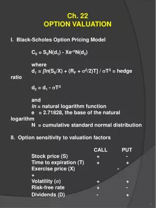
Black-Scholes Option Pricing Model • The Black-Scholes model was originally developed to price call options • N(d1) and N(d2) are found using the cumulative standard normal distribution tables
Example: OPM • You are looking at a call option with 6 months to expiration and an exercise price of $35. The current stock price is $45 and the risk-free rate is 4%. The standard deviation of underlying asset returns is 20%. What is the value of the call option? • Look up N(d1) and N(d2) in Table 24.3 • N(d1) = (.9761+.9772)/2 = .9767 • N(d2) = (.9671+.9686)/2 = .9679 C = 45(.9767) – 35e-.04(.5)(.9679) C = $10.75
Example: OPM in a Spreadsheet • Consider the previous example • Click on the excel icon to see how this problem can be worked in a spreadsheet
Put Values • The value of a put can be found by finding the value of the call and then using put-call parity • What is the value of the put in the previous example? • P = C + Ee-Rt – S • P = 10.75 + 35e-.04(.5) – 45 = .06 • Note that a put may be worth more if exercised than if sold, while a call is worth more “alive than dead” unless there is a large expected cash flow from the underlying asset
European vs. American Options • The Black-Scholes model is strictly for European options • It does not capture the early exercise value that sometimes occurs with a put • If the stock price falls low enough, we would be better off exercising now rather than later • A European option will not allow for early exercise and therefore, the price computed using the model will be too low relative to that of an American option that does allow for early exercise
Varying Stock Price and Delta • What happens to the value of a call (put) option if the stock price changes, all else equal? • Take the first derivative of the OPM with respect to the stock price and you get delta. • For calls: Delta = N(d1) • For puts: Delta = N(d1) - 1 • Delta is often used as the hedge ratio to determine how many options we need to hedge a portfolio
Work the Web Example • There are several good options calculators on the Internet • Click on the web surfer to go to ivolatility.com and click on the Basic Calculator under Analysis Tools • Price the call option from the earlier example • S = $45; E = $35; R = 4%; t = .5; = .2 • You can also choose a stock and value options on a particular stock
Example: Delta • Consider the previous example: • What is the delta for the call option? What does it tell us? • N(d1) = .9767 • The change in option value is approximately equal to delta times the change in stock price • What is the delta for the put option? • N(d1) – 1 = .9767 – 1 = -.0233 • Which option is more sensitive to changes in the stock price? Why?
Varying Time to Expiration and Theta • What happens to the value of a call (put) as we change the time to expiration, all else equal? • Take the first derivative of the OPM with respect to time and you get theta • Options are often called “wasting” assets, because the value decreases as expiration approaches, even if all else remains the same • Option value = intrinsic value + time premium
Example: Time Premiums • What was the time premium for the call and the put in the previous example? • Call • C = 10.75; S = 45; E = 35 • Intrinsic value = max(0, 45 – 35) = 10 • Time premium = 10.75 – 10 = $0.75 • Put • P = .06; S = 45; E = 35 • Intrinsic value = max(0, 35 – 45) = 0 • Time premium = .06 – 0 = $0.06
Varying Standard Deviation and Vega • What happens to the value of a call (put) when we vary the standard deviation of returns, all else equal? • Take the first derivative of the OPM with respect to sigma and you get vega • Option values are very sensitive to changes in the standard deviation of return • The greater the standard deviation, the more the call and the put are worth • You loss is limited to the premium paid, more volatility increases your potential gain
Varying the Risk-Free Rate and Rho • What happens to the value of a call (put) as we vary the risk-free rate, all else equal? • The value of a call increases • The value of a put decreases • Take the first derivative of the OPM with respect to the risk-free rate and you get rho • Changes in the risk-free rate have very little impact on options values over any normal range of interest rates
Implied Standard Deviations • All of the inputs into the OPM are directly observable, except for the expected standard deviation of returns • The OPM can be used to compute the market’s estimate of future volatility by solving for the standard deviation • This is called the implied standard deviation • Online options calculators are useful for this computation since there is not a closed form solution
Work the Web Example • Use the options calculator at www.numa.com to find the implied volatility of a stock of your choice • Click on the web surfer to go to finance.yahoo.com to get the required information • Click on the web surfer to go to numa, enter the information and find the implied volatility
Equity as a Call Option • Equity can be viewed as a call option on the firm’s assets whenever the firm carries debt • The strike price is the cost of making the debt payments • The underlying asset price is the market value of the firm’s assets • If the intrinsic value is positive, the firm can exercise the option by paying off the debt • If the intrinsic value is negative, the firm can let the option expire and turn the firm over to the bondholders • This concept is useful in valuing certain types of corporate decisions
Valuing Equity and Changes in Assets • Consider a firm that has a zero-coupon bond that matures in 4 years. The face value is $30 million and the risk-free rate is 6%. The current market value of the firm’s assets is $40 million and the firm’s equity is currently worth $18 million. Suppose the firm is considering a project with an NPV = $500,000. • What is the implied standard deviation of returns? • What is the delta? • What is the change in stockholder value?
PCP and the Balance Sheet Identity • Risky debt can be viewed as a risk-free bond minus the cost of a put option • Value of risky bond = Ee-Rt – P • Consider the put-call parity equation and rearrange • S = C + Ee-Rt – P • Value of assets = value of equity + value of a risky bond • This is just the same as the traditional balance sheet identity • Assets = liabilities + equity
Mergers and Diversification • Diversification is a frequently mentioned reason for mergers • Diversification reduces risk and therefore volatility • Decreasing volatility decreases the value of an option • Assume diversification is the only benefit to a merger • Since equity can be viewed as a call option, should the merger increase or decrease the value of the equity? • Since risky debt can be viewed as risk-free debt minus a put option, what happens to the value of the risky debt? • Overall, what has happened with the merger and is it a good decision in view of the goal of stockholder wealth maximization?
Extended Example – Part I • Consider the following two merger candidates • The merger is for diversification purposes only with no synergies involved • Risk-free rate is 4%
Extended Example – Part II • Use the OPM (or an options calculator) to compute the value of the equity • Value of the debt = value of assets – value of equity
Extended Example – Part III • The asset return standard deviation for the combined firm is 30% • Market value assets (combined) = 40 + 15 = 55 • Face value debt (combined) = 18 + 7 = 25 Total MV of equity of separate firms = 25.681 + 9.867 = 35.548 Wealth transfer from stockholders to bondholders = 35.548 – 34.120 = 1.428 (exact increase in MV of debt)
M&A Conclusions • Mergers for diversification only transfer wealth from the stockholders to the bondholders • The standard deviation of returns on the assets is reduced, thereby reducing the option value of the equity • If management’s goal is to maximize stockholder wealth, then mergers for reasons of diversification should not occur
Extended Example: Low NPV – Part I • Stockholders may prefer low NPV projects to high NPV projects if the firm is highly leveraged and the low NPV project increases volatility • Consider a company with the following characteristics • MV assets = 40 million • Face Value debt = 25 million • Debt maturity = 5 years • Asset return standard deviation = 40% • Risk-free rate = 4%
Extended Example: Low NPV – Part II • Current market value of equity = $22.657 million • Current market value of debt = $17.343 million
Extended Example: Low NPV – Part III • Which project should management take? • Even though project B has a lower NPV, it is better for stockholders • The firm has a relatively high amount of leverage • With project A, the bondholders share in the NPV because it reduces the risk of bankruptcy • With project B, the stockholders actually appropriate additional wealth from the bondholders for a larger gain in value
Extended Example: Negative NPV – Part I • We’ve seen that stockholders might prefer a low NPV to a high one, but would they ever prefer a negative NPV? • Under certain circumstances, they might • If the firm is highly leveraged, stockholders have nothing to lose if a project fails and everything to gain if it succeeds • Consequently, they may prefer a very risky project with a negative NPV but high potential rewards
Extended Example: Negative NPV – Part II • Consider the previous firm • They have one additional project they are considering with the following characteristics • Project NPV = -$2 million • MV of assets = $38 million • Asset return standard deviation = 65% • Estimate the value of the debt and equity • MV equity = $25.423 million • MV debt = $12.577 million
Extended Example: Negative NPV – Part III • In this case, stockholders would actually prefer the negative NPV project to either of the positive NPV projects • The stockholders benefit from the increased volatility associated with the project even if the expected NPV is negative • This happens because of the large levels of leverage
Conclusions • As a general rule, managers should not go around accepting low or negative NPV projects and passing up high NPV projects • Under certain circumstances, however, this may benefit stockholders • The firm is highly leveraged • The low or negative NPV project causes a substantial increase in the standard deviation of asset returns
Quick Quiz • What is put-call parity? What would happen if it doesn’t hold? • What is the Black-Scholes option pricing model? • How can equity be viewed as a call option? • Should a firm do a merger for diversification purposes only? Why or why not? • Should management ever accept a negative NPV project? If yes, under what circumstances?
24 End of Chapter