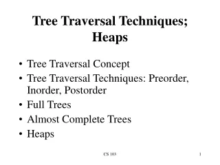
Tree Traversal Techniques; Heaps
Explore the concept of tree traversal techniques including Preorder, Inorder, and Postorder with illustrations and code examples in CS 103.

Tree Traversal Techniques; Heaps
E N D
Presentation Transcript
Tree Traversal Techniques; Heaps • Tree Traversal Concept • Tree Traversal Techniques: Preorder, Inorder, Postorder • Full Trees • Almost Complete Trees • Heaps CS 103
1 3 7 5 8 9 4 6 11 12 Binary-Tree Related Definitions • The children of any node in a binary tree are ordered into a left child and a right child • A node can have a left and a right child, a left child only, a right child only, or no children • The tree made up of a left child (of a node x) and all its descendents is called the left subtree of x • Right subtrees are defined similarly 10 CS 103
A Binary-tree Node Class class TreeNode { public: typedef int datatype; TreeNode(datatype x=0, TreeNode *left=NULL, TreeNode *right=NULL){ data=x; this->left=left; this->right=right; }; datatype getData( ) {return data;}; TreeNode *getLeft( ) {returnleft;}; TreeNode *getRight( ) {returnright;}; void setData(datatype x) {data=x;}; void setLeft(TreeNode *ptr) {left=ptr;}; void setRight(TreeNode *ptr) {right=ptr;}; private: datatype data; // different data type for other apps TreeNode *left; // the pointer to left child TreeNode *right; // the pointer to right child }; CS 103
Binary Tree Class class Tree { public: typedef int datatype; Tree(TreeNode *rootPtr=NULL){this->rootPtr=rootPtr;}; TreeNode *search(datatype x); bool insert(datatype x); TreeNode * remove(datatype x); TreeNode *getRoot(){return rootPtr;}; Tree *getLeftSubtree(); Tree *getRightSubtree(); bool isEmpty(){return rootPtr == NULL;}; private: TreeNode *rootPtr; }; CS 103
Binary Tree Traversal • Traversal is the process of visiting every node once • Visiting a node entails doing some processing at that node, but when describing a traversal strategy, we need not concern ourselves with what that processing is CS 103
Binary Tree Traversal Techniques • Three recursive techniques for binary tree traversal • In each technique, the left subtree is traversed recursively, the right subtree is traversed recursively, and the root is visited • What distinguishes the techniques from one another is the order of those 3 tasks CS 103
Preoder, Inorder, Postorder • Preorder Traversal: • Visit the root • Traverse left subtree • Traverse right subtree • In Preorder, the root is visited before (pre) the subtrees traversals • In Inorder, the root is visited in-between left and right subtree traversal • In Preorder, the root is visited after (pre) the subtrees traversals • Inorder Traversal: • Traverse left subtree • Visit the root • Traverse right subtree • Postorder Traversal: • Traverse left subtree • Traverse right subtree • Visit the root CS 103
1 3 7 10 5 8 9 4 6 11 12 Illustrations for Traversals • Assume: visiting a node is printing its label • Preorder: 1 3 5 4 6 7 8 9 10 11 12 • Inorder: 4 5 6 3 1 8 7 9 11 10 12 • Postorder: 4 6 5 3 8 11 12 10 9 7 1 CS 103
15 20 8 27 11 2 30 6 22 10 12 3 7 14 Illustrations for Traversals (Contd.) • Assume: visiting a node is printing its data • Preorder: 15 8 2 6 3 7 11 10 12 14 20 27 22 30 • Inorder: 2 3 6 7 8 10 11 12 14 15 20 22 27 30 • Postorder: 3 7 6 2 10 14 12 11 8 22 30 27 20 15 CS 103
Code for the Traversal Techniques void preOrder(Tree *tree){ if (tree->isEmpty( )) return; visit(tree->getRoot( )); preOrder(tree->getLeftSubtree()); preOrder(tree->getRightSubtree()); } • The code for visit is up to you to provide, depending on the application • A typical example for visit(…) is to print out the data part of its input node void inOrder(Tree *tree){ if (tree->isEmpty( )) return; inOrder(tree->getLeftSubtree( )); visit(tree->getRoot( )); inOrder(tree->getRightSubtree( )); } void postOrder(Tree *tree){ if (tree->isEmpty( )) return; postOrder(tree->getLeftSubtree( )); postOrder(tree->getRightSubtree( )); visit(tree->getRoot( )); } CS 103
Application of Traversal Sorting a BST • Observe the output of the inorder traversal of the BST example two slides earlier • It is sorted • This is no coincidence • As a general rule, if you output the keys (data) of the nodes of a BST using inorder traversal, the data comes out sorted in increasing order CS 103
Other Kinds of Binary Trees(Full Binary Trees) • Full Binary Tree: A full binary tree is a binary tree where all the leaves are on the same level and every non-leaf has two children • The first four full binary trees are: CS 103
Examples of Non-Full Binary Trees • These trees are NOT full binary trees: (do you know why?) CS 103
1 1 1 3 3 2 2 6 4 5 7 1 2 3 5 6 7 4 11 8 9 10 13 14 15 12 Canonical Labeling ofFull Binary Trees • Label the nodes from 1 to n from the top to the bottom, left to right Relationships between labels of children and parent: i 2i+1 2i CS 103
Other Kinds of Binary Trees(Almost Complete Binary trees) • Almost Complete Binary Tree: An almost complete binary tree of n nodes, for any arbitrary nonnegative integer n, is the binary tree made up of the first n nodes of a canonically labeled full binary 1 1 1 1 1 2 3 2 3 2 2 1 6 4 5 1 4 2 3 2 3 4 5 6 4 5 7 CS 103
Depth/Height of Full Trees and Almost Complete Trees • The height (or depth ) h of such trees is O(log n) • Proof: In the case of full trees, • The number of nodes n is: n=1+2+22+23+…+2h=2h+1-1 • Therefore, 2h+1 = n+1, and thus, h=log(n+1)-1 • Hence, h=O(log n) • For almost complete trees, the proof is left as an exercise. CS 103
Canonical Labeling ofAlmost Complete Binary Trees • Same labeling inherited from full binary trees • Same relationship holding between the labels of children and parents: Relationships between labels of children and parent: i 2i+1 2i CS 103
Array Representation of Full Trees and Almost Complete Trees • A canonically label-able tree, like full binary trees and almost complete binary trees, can be represented by an array A of the same length as the number of nodes • A[k] is identified with node of label k • That is, A[k] holds the data of node k • Advantage: • no need to store left and right pointers in the nodes save memory • Direct access to nodes: to get to node k, access A[k] CS 103
Illustration of Array Representation 15 20 8 • Notice: Left child of A[5] (of data 11) is A[2*5]=A[10] (of data 18), and its right child is A[2*5+1]=A[11] (of data 12). • Parent of A[4] is A[4/2]=A[2], and parent of A[5]=A[5/2]=A[2] 30 2 11 27 13 18 12 6 2 30 8 20 11 6 10 15 27 12 13 8 9 10 11 1 2 3 4 5 6 7 CS 103
Adjustment of Indexes • Notice that in the previous slides, the node labels start from 1, and so would the corresponding arrays • But in C/C++, array indices start from 0 • The best way to handle the mismatch is to adjust the canonical labeling of full and almost complete trees. • Start the node labeling from 0 (rather than 1). • The children of node k are now nodes (2k+1) and (2k+2), and the parent of node k is (k-1)/2, integer division. CS 103
Application of Almost Complete Binary Trees: Heaps • A heap (or min-heap to be precise) is an almost complete binary tree where • Every node holds a data value (or key) • The key of every node is ≤ the keys of the children Note: A max-heap has the same definition except that the Key of every node is >= the keys of the children CS 103
Example of a Min-heap 5 20 8 30 15 11 27 16 18 12 33 CS 103
Operations on Heaps • Delete the minimum value and return it. This operation is called deleteMin. • Insert a new data value • Applications of Heaps: • A heap implements a priority queue, which is a queue • that orders entities not a on first-come first-serve basis, • but on a priority basis: the item of highest priority is at • the head, and the item of the lowest priority is at the tail • Another application: sorting, which will be seen later CS 103
DeleteMin in Min-heaps • The minimum value in a min-heap is at the root! • To delete the min, you can’t just remove the data value of the root, because every node must hold a key • Instead, take the last node from the heap, move its key to the root, and delete that last node • But now, the tree is no longer a heap (still almost complete, but the root key value may no longer be ≤ the keys of its children CS 103
5 20 8 30 15 11 27 16 18 12 33 Illustration of First Stage of deletemin 20 8 30 15 11 27 16 12 18 33 12 12 20 8 20 8 30 15 11 27 30 15 11 27 16 18 33 16 18 33 CS 103
Restore Heap • To bring the structure back to its “heapness”, we restore the heap • Swap the new root key with the smaller child. • Now the potential bug is at the one level down. If it is not already ≤ the keys of its children, swap it with its smaller child • Keep repeating the last step until the “bug” key becomes ≤ its children, or the it becomes a leaf CS 103
Illustration of Restore-Heap 12 8 20 20 8 12 30 30 15 11 27 15 11 27 16 16 18 18 33 33 8 20 11 30 15 12 27 16 18 Now it is a correct heap 33 CS 103
Time complexity of insert and deletmin • Both operations takes time proportional to the height of the tree • When restoring the heap, the bug moves from level to level until, in the worst case, it becomes a leaf (in deletemin) or the root (in insert) • Each move to a new level takes constant time • Therefore, the time is proportional to the number of levels, which is the height of the tree. • But the height is O(log n) • Therefore, both insert and deletemin take O(log n) time, which is very fast. CS 103
Inserting into a minheap • Suppose you want to insert a new value x into the heap • Create a new node at the “end” of the heap (or put x at the end of the array) • If x is >= its parent, done • Otherwise, we have to restore the heap: • Repeatedly swap x with its parent until either x reaches the root of x becomes >= its parent CS 103
Illustration of Insertion Into the Heap • In class CS 103
The Min-heap Class in C++ class Minheap{ //the heap is implemented with a dynamic array public: typedef int datatype; Minheap(int cap = 10){capacity=cap; length=0; ptr = new datatype[cap];}; datatype deleteMin( ); void insert(datatype x); bool isEmpty( ) {return length==0;}; int size( ) {return length;}; private: datatype *ptr; // points to the array int capacity; int length; void doubleCapacity(); //doubles the capacity when needed }; CS 103
Code for deletemin Minheap::datatype Minheap::deleteMin( ){ assert(length>0); datatype returnValue = ptr[0]; length--; ptr[0]=ptr[length]; // move last value to root element int i=0; while ((2*i+1<length && ptr[i]>ptr[2*i+1]) || (2*i+2<length && (ptr[i]>ptr[2*i+1] || ptr[i]>ptr[2*i+2]))){ // “bug” still > at least one child if (ptr[2*i+1] <= ptr[2*i+2]){ // left child is the smaller child datatype tmp= ptr[i]; ptr[i]=ptr[2*i+1]; ptr[2*i+1]=tmp; //swap i=2*i+1; } else{ // right child if the smaller child. Swap bug with right child. datatype tmp= ptr[i]; ptr[i]=ptr[2*i+2]; ptr[2*i+2]=tmp; // swap i=2*i+2; } } return returnValue; }; CS 103
Code for Insert void Minheap::insert(datatype x){ if (length==capacity) doubleCapacity(); ptr[length]=x; int i=length; length++; while (i>0 && ptr[i] < ptr[i/2]){ datatype tmp= ptr[i]; ptr[i]=ptr[(i-1)/2]; ptr[(i-1)/2]=tmp; i=(i-1)/2; } }; CS 103
Code for doubleCapacity void Minheap::doubleCapacity(){ capacity = 2*capacity; datatype *newptr = new datatype[capacity]; for (int i=0;i<length;i++) newptr[i]=ptr[i]; delete [] ptr; ptr = newptr; }; CS 103