Download
1 / 27
270 likes | 286 Vues
This project aims to create a traffic atlas of LA using empirical data to highlight trends and problem areas, providing a straightforward representation for the public. Methods include MatLab scripting and data analysis to calculate Travel Time Index. Challenges include data gaps and technical difficulties. Results show traffic trends, but further analysis is needed for conclusive insights. Future steps include expanding data and user testing for improved usability.

E N D
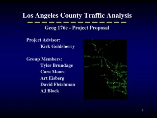
Los Angeles County Traffic Analysis Geog 176c - Project Proposal Project Advisor: Kirk Goldsberry Group Members: Tyler Brundage Cara Moore Art Eisberg David Fleishman AJ Block
Objectives • Create a traffic atlas using empirical data • Supplement perceptions of LA traffic
Objectives • Depict traffic trends in LA using a GIS • Highlight problem areas and time periods • Create a straightforward representation for the general public
Final Product http://www.geog.ucsb.edu/~ccm176/
Methods • Outsourced MatLab scripting • Calculated Average Velocity with MatLab • Imported .txt files into Excel
Methods • Imported Excel files to Access • Used Common Key to Link Velocities by Sensor ID number • Caluclated TTI in Excel • (Average Freeflow Velocity/ Average Velocity at Certain Time) • Exported file as a .dbf
Travel Time Index • In layman’s terms, the TTI indicates how much longer a trip would take than it would in free-flow conditions • If TTI = 1, the trip would take the same amount of time as free flow traffic • If TTI = 2, the trip would take twice as long
Methods • Calculated Average TTI for each Day/Time to make graphs • Merged Highways • Joined .dbf files to Highways
Methods • Decided on Class Breaks/ Color Schemes • Created Maps in ArcMap • Created Flash File & Published Web Page
Problems • Gaps in data • Data Spread • Excel prior to 2007 can only have 256 columns • Lack of data • Only used January
Problems • Technical difficulties • -99s= non functioning sensors • TTI may not be intuitive
Problems • Large amount of data • 1368 Rows • 205 Maps • 280,440 lines in Flash • 10 minutes to open Flash File • 1 ½ hour plus to export file
Interpreting Results • There appears to be a definite trend of traffic throughout the day • Rush Hour • Northbound/Southbound & Eastbound/Westbound trends • However, there also appears to be many anomalies • Likely due to the spread of data used
Background Research * Y-axis indicates the fraction of sensors indicating congestion From http://home.znet.com/schester/calculations/traffic/la/index.html
Graph 19
Interpreting Results • We have yet to test the efficiency of the final map • Therefore, we do not know how intuitive the final product is
Conclusions • While a general trend associated with time and day can be seen, no conclusions should be made without a more in depth analysis using a larger data spread
Future • Use more data to provide more conclusive results • More days • More times (e.g. every 5 minutes)
Future • Test final product with general public • Based on public input, edit map to make it more user friendly
Future • Develop Algorithm using TTI so services like MapQuest could provide time estimations from point A to point B