Nonparametric Survey Regression Estimation Using Penalized Splines
Nonparametric Survey Regression Estimation Using Penalized Splines. F. Jay Breidt *,** Colorado State University Jean D. Opsomer ** Iowa State University (+ more folks acknowledged soon) Research supported by EPA STAR Grants R-82909501 (*CSU) and R-82909601 (**OSU). The Usual Disclaimer.


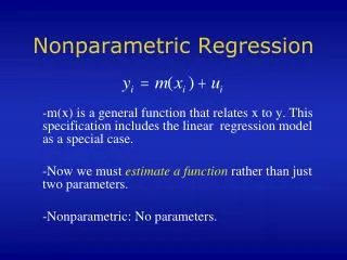
Nonparametric Survey Regression Estimation Using Penalized Splines
E N D
Presentation Transcript
Nonparametric Survey Regression Estimation Using Penalized Splines F. Jay Breidt*,** Colorado State University Jean D. Opsomer** Iowa State University (+ more folks acknowledged soon) Research supported by EPA STAR Grants R-82909501 (*CSU) and R-82909601 (**OSU)
The Usual Disclaimer • The work reported here was developed under STAR Research Assistance Agreements CR-829095 and CR-829096 awarded by the U.S. Environmental Protection Agency (EPA) to Colorado State University and Oregon State University. This presentation has not been formally reviewed by EPA. The views expressed here are solely those of the authors. EPA does not endorse any products or commercial services mentioned in this report.
Outline • Background: • Scales of inference • Specific versus generic • Model-assisted and model-based inference • Penalized splines: • Comparison to other smoothers; two-stage; small area • Variations: network data, increment data • Other: • Non-Gaussian time series • Summary: • Status of STARMAP.2 and DAMARS.5
Scales of Inference in Surveys • Large area: • sample itself suffices for inference • no model needed • Medium area: • use auxiliary information through a model • model helps inference but is not critical • Small area: • sample size is small or zero • inference must be based on a model
Specific and Generic Inference • Specific: one study variable, few population parameters • lots of modeling resources to specify, estimate, and diagnose a model • willingness to defend the model • Generic: many study variables, many population parameters • no resources to model every variable • no single model is adequate/defensible
Generic Inferences in Aquatic Resources • Generic inference is a common problem for federal, state, and tribal agencies • Example: conduct a survey and prepare a report • analyze large numbers of chemical, biological, and physical variables • estimate means, quantiles, and distribution functions • break down both by political classifications and by various ecological classifications
Model-Assisted Survey Inference • Scarce modeling resources for generic inference, so we don’t trust models • Can we use a model without depending on the model? • Model-assisted inference: • efficiency gains if model is right • sensible inference even if model is wrong
Model-Assisted Estimators • Form of model-assisted estimator: • (model-based prediction)+(design bias adjustment) • model incorporates auxiliary information • bias adjustment corrects for bad models • Classical parametric model-assisted: • prediction from linear regression model • Our idea: nonparametric model-assisted • prediction fromkernel regression or other “smoother” (JB & JO (2000), Annals of Stat)
Why Nonparametric? • More flexible model specification • smooth mean function, positive variance function • Approximately correct more often • more opportunities for efficiency gains from auxiliary information • often, not a large efficiency loss if parametric specification is correct
Goals of Our Research • Focus on generic inference • Use flexible nonparametric models to reduce misspecification bias • model-assisted: medium area problem • model-based: small area problem • Make the methods operationally feasible for state and tribal agencies • linear smoothers generate generic weights
Penalized Splines • Very useful class of linear smoothers • Readily fits into standard linear mixed model framework • Modular, extensible, computationally convenient • Automated smoothing parameter selection and fitting with standard software • Several ongoing projects: • Model-assisted p-spline estimation (Gerda Claeskens, JO, JB); two-stage extensions (Mark Delorey) • Small area p-spline estimation (Gerda, Giovanna Ranalli, Goran Kauermann, JO, JB) • Smoothing on networks (Giovanna, JB) • Semiparametric mixed models for increment-averaged core data (Nan-Jung Hsu, Steve Ogle, JB)
Penalized Splines • Truncated linear basis allows slope changes at each of many knots: • Penalize for unnecessary slope changes:
P-Splines: Influence of Penalty • Fits with increasing penalty parameter
Penalized Splines Computation • Computation using S-Plus • Set up design matrix + truncated linear splines Z <- outer(x, knots, "-") Z <- Z * (Z > 0) C <- cbind(one,x,Z) • Solve for spline with fixed degrees of freedom D <- diag(rep(0,2),rep(1,K)) mhat <- X %*% solve(t(C) %*% diag(1/pi) %*% C +lambda^2 * D) %*% t(C) %*% diag(1/pi)%*%y • For data-determined df/roughness penalty, can use lme()to select via REML
Model-Assisted P-Spline Estimator • Model-based prediction + design bias adjustment: • Asymptotically design-unbiased and design consistent • Asymptotic variance given by
Design of Simulation Study • Model-assisted estimators • Polynomial regression • Poststratification (piecewise constant) • Local polynomial regression (kernel) • Penalized spline • Model-based estimator • Penalized spline • All use common degrees of freedom: 3 or 6 • Eight response variables on one population • Two noise levels • N=1000 • Designs SI or STSI • 1000 replicate samples of size n=50
Further Results from Simulation • Variance estimation • For all estimators, variance estimator has negative bias • Weighted residual variance estimator performs better • Confidence interval coverage • Somewhat less than nominal for all estimators (90-92%) • Undercoverage not as severe as bias would suggest • Negative weights: (2 df)x(2 designs)x(1000 reps)x(50 weights) = 200,000 weights • 902 negative REG weights • 145 negative LLR weights • 2 negative MA weights
Two-Stage P-Spline Estimation • Available auxiliary information in two-stage sampling: • All clusters • All elements • All elements in sampled clusters • Mark Delorey (poster): focus on first case • Simulation study comparing Horvitz-Thompson, regression, model-based p-spline, model-assisted p-spline with and without cluster random effects • Operational issues with df, cluster variance component • Some results: p-spline is good!
Semiparametric Small Area Estimation • Gerda, Giovanna, Goran Kauermann, JO, JB • Example: ANC level for Northeastern lakes • 557 observations over 113 HUCs • Average sample size/HUC: 4.9 • 64 HUCs contain less than 5 observations • Site-specific covariates: lake location and elevation • Simple way to capture spatial effects?
Semiparametric Small Area Model • Replace linear function of covariates by more general model: • direct estimator = truth + sampling error • truth = semiparametric regression + area-specific deviation • Semiparametric regression expressed as linear mixed model • Thin plate splines • Low-rank radial basis functions
Small Area Estimation Results • EBLUP for this model easily handled with standard software (SAS proc mixed, SPlus lme())
P-Splines for Increment Data • Common for soil, sediment core data: • Datum represents not a single depth point but a depth increment (e.g., cylinder of soil 2.5cm in diameter x 15cm high, collected at 20-35 cm) • Ignoring increment structure leads to biased, inconsistent estimators • Integrate linear mixed model representation: • Definite integral of truncated linear basis (x-κ)+becomes differenced quadratic basis [(top-κ)+ ]2 - [(bottom-κ)+ ]2 • Immediate extension to small area estimation • E.g., soil mapping by map unit symbol
Carbon Sequestration • (Nan-Jung Hsu, Steve Ogle, JB) Broad class of semiparametric mixed models for increment-averaged data
Smoothing on Networks • Current research with post-doc, Giovanna Ranalli • have noisy data on stream network • have within-network distance measure (rather than “as the crow flies”) • want interpolations at unsampled locations in network • Semiparametric methodology readily extends to this setting • low-rank radial basis functions • Possible real data from EPA (John Faustini)
Smoothing on Stream Networks • Toy stream network • Two first-order, one second-order stream segment • Regression function is exponential along straight reach (two segments), constant along remaining segment, continuous at intersection • n=150 noisy observations obtained along network
Toy Network Results • Noisy observations smoothed via • Low-rank thin plate spline (2D, ignoring network structure) • Within-network radial basis functions (1D, accounts for network structure) • Network smooth offers 25-30% reduction in MISE over spatial smooth
Non-Gaussian Time Series • Potential models for one-dimensional spatial processes
Identification and Estimation • In Gaussian case, models of differing causality/invertibility cannot be identified • Identification in non-Gaussian case: • Fit causal/invertible ARMA via Gaussian quasi-MLE • Examine residuals for IID-ness • If not IID, fit All-Pass model (LAD [Breidt, Davis, Trindade, Ann. Stat. (2001)], MLE, rank estimation) to determine order of non-causality or non-invertibility • Prediction and Estimation in non-Gaussian case: • Best MS prediction requires trickery • Exact MLE, Bayes for non-Gaussian MA • Exact and conditional MLE for MA with roots near unit circle [Rosenblatt, Davis, Breidt, Hsu]
Where Are We Now? • DAMARS.5: Nonparametric model-assisted • 1. Extensions • 1.1 continuous spatial domains (Siobhan;poster; Giovanna, work in progress) • 1.2 multiple phases (Kim (PhD 2004, ISU), working paper) • 1.3 multiple auxiliary variables (gam: Gretchen, Goran, JO, JB, JASA 2nd submission) • 1.3-1.4 alternative smoothing (Gerda, JO, JB, p-splines;Biometrika 2ndsubmission; Ranalli and Montanari, neural nets, JASA 2nd submission) • Other: two-stage kernels (Kim, JO, JB;JRSS submission); two-stage splines (Mark, JB, poster) • 2. Applications • 2.1 CDF estimation (Alicia, JO, JB;poster, CJS submission) • 2.2 “Medium” area (Siobhan, JO, JB;poster) • 2.3 Surveys over time (Jehad Al-Jararha, JO, JB, spam with partial overlap;) • 2.4 Nonresponse (da Silva and Opsomer, Survey Methodology 2004)
Where Are We Now? • STARMAP.2: Local Inferences • 1. Small area • 1.1-1.4 Nonparametric model-assisted for spatial (Siobhan, poster; Giovanna, work in progress); Semiparametric (Gerda, Giovanna, Goran, JO, JB, working paper); Increments (Nan-Jung, Steve, JB, working paper) • 1.1 MLE for all-pass (Beth, RD, JB, JMVA submission) ; rank for all-pass (Beth, RD, JB, working paper); Prediction for MA (Breidt and Hsu, Stat Sinica 2004); Exact MLE for MA (Nan-Jung, RD, JB) • Spatial trend detection (Hsin-Cheng Huang) • Design aspects: (Bill, JB, poster) • 2. Deconvolution • Formulated as another small area estimation problem using constrained Bayes methods (Mark,JB, poster) • Methodology seems OK; example (88 HUCs in MAHA) still being tweaked; work in progress • 3. Causal inference • 3.1-3.3 (Alix G)
Some Summaries (these projects only) • Some Invited Talks and Seminars • Winemiller Symposium (Columbia, MO) • Computational Environmetrics (Chicago, IL) • Monitoring Symposium (Denver, CO) • ICSA (Singapore) • EMAP 2004 (Newport, RI) • ENAR (Pittsburgh PA) • IWAP (Piraeus, Greece) • IMS-ASA (Calcutta, India) • Western Ecology Division, EPA (Corvallis, OR) • University of Maryland (Baltimore County, MD) • + Jean’s talks
More Summaries (these projects only) • People • Students: Ji-Yeon Kim, ISU PhD completed Spring 2004 (JO and JB); Bill Coar, Mark Delorey, Jehad Al-Jararha, CSU PhD work in progress; ISU student? • Post-Doctoral Research Associate: Giovanna Ranalli • Visiting Research Scientists: Nan-Jung Hsu and Hsin-Cheng Huang • Unsuspecting Collaborators: Gerda Claeskens and Goran Kauermann • Papers • 2 appeared, 2 tentatively accepted, 1 invited revision, 4 submitted, n working papers
Optimal Sampling Design under Frame Imperfections • Motivated by problems with RF3 perennial classification • About 20% errors of omission and of commission! • Previous work: logistic regression for probability of perennial as function of covariates (Bill Coar) • Compare optimal biased and unbiased designs using anticipated MSE criterion • Account for differential costs (in frame, not in frame; perennial, non-perennial) • Minimize AMSE for fixed cost • Further work • Asymptotic results for cases of negligible, non-negligible bias • Empirical results