Data Mining, Data Warehousing and Knowledge Discovery Basic Algorithms and Concepts
Data Mining, Data Warehousing and Knowledge Discovery Basic Algorithms and Concepts. Srinath Srinivasa IIIT Bangalore sri@iiitb.ac.in. Overview. Why Data Mining? Data Mining concepts Data Mining algorithms Tabular data mining Association, Classification and Clustering

Data Mining, Data Warehousing and Knowledge Discovery Basic Algorithms and Concepts
E N D
Presentation Transcript
Data Mining, Data Warehousing and Knowledge DiscoveryBasic Algorithms and Concepts Srinath Srinivasa IIIT Bangalore sri@iiitb.ac.in
Overview • Why Data Mining? • Data Mining concepts • Data Mining algorithms • Tabular data mining • Association, Classification and Clustering • Sequence data mining • Streaming data mining • Data Warehousing concepts
Why Data Mining From a managerial perspective: Analyzing trends Wealth generation Security Strategic decision making
Data Mining • Look for hidden patterns and trends in data that is not immediately apparent from summarizing the data • No Query… • …But an “Interestingness criteria”
Data Mining + = Interestingness criteria Hidden patterns Data
Data Mining Type of Patterns + = Interestingness criteria Hidden patterns Data
Data Mining Type of data Type of Interestingness criteria + = Interestingness criteria Hidden patterns Data
Type of Data • Tabular (Ex: Transaction data) • Relational • Multi-dimensional • Spatial (Ex: Remote sensing data) • Temporal (Ex: Log information) • Streaming (Ex: multimedia, network traffic) • Spatio-temporal (Ex: GIS) • Tree (Ex: XML data) • Graphs (Ex: WWW, BioMolecular data) • Sequence (Ex: DNA, activity logs) • Text, Multimedia …
Type of Interestingness • Frequency • Rarity • Correlation • Length of occurrence (for sequence and temporal data) • Consistency • Repeating / periodicity • “Abnormal” behavior • Other patterns of interestingness…
Data Mining vs Statistical Inference Statistics: Statistical Reasoning Conceptual Model (Hypothesis) “Proof” (Validation of Hypothesis)
Data Mining vs Statistical Inference Data mining: Mining Algorithm Based on Interestingness Data Pattern (model, rule, hypothesis) discovery
Data Mining Concepts Associations and Item-sets: An association is a rule of the form: if X then Y. It is denoted as X Y Example: If India wins in cricket, sales of sweets go up. For any rule if X Y Y X, then X and Y are called an “interesting item-set”. Example: People buying school uniforms in June also buy school bags (People buying school bags in June also buy school uniforms)
Data Mining Concepts Support and Confidence: The support for a rule R is the ratio of the number of occurrences of R, given all occurrences of all rules. The confidence of a rule X Y, is the ratio of the number of occurrences of Y given X, among all other occurrences given X.
Data Mining Concepts Support and Confidence: Support for {Bag, Uniform} = 5/10 = 0.5 Confidence for Bag Uniform = 5/8 = 0.625 Bag Books Bag Bag Uniform Bag Crayons Books Uniform Pencil Uniform Bag Uniform Pencil Crayons Pencil Uniform Crayons Crayons Uniform Crayons Uniform Pencil Book Bag Book Bag Bag Pencil Books
Mining for Frequent Item-sets • The Apriori Algorithm: • Given minimum required support s as interestingness criterion: • Search for all individual elements (1-element item-set) that have a minimum support of s • Repeat • From the results of the previous search for i-element item-sets, search for all i+1 element item-sets that have a minimum support of s • This becomes the set of all frequent (i+1)-element item-sets that are interesting • Until item-set size reaches maximum..
Mining for Frequent Item-sets The Apriori Algorithm: (Example) Let minimum support = 0.3 Interesting 1-element item-sets: {Bag}, {Uniform}, {Crayons}, {Pencil}, {Books} Interesting 2-element item-sets: {Bag,Uniform} {Bag,Crayons} {Bag,Pencil} {Bag,Books} {Uniform,Crayons} {Uniform,Pencil} {Pencil,Books} Bag Books Bag Bag Uniform Bag Crayons Books Uniform Pencil Uniform Bag Uniform Pencil Crayons Pencil Uniform Crayons Crayons Uniform Crayons Uniform Pencil Books Bag Books Bag Bag Pencil Books
Mining for Frequent Item-sets The Apriori Algorithm: (Example) Let minimum support = 0.3 Interesting 3-element item-sets: {Bag,Uniform,Crayons} Bag Books Bag Bag Uniform Bag Crayons Books Uniform Pencil Uniform Bag Uniform Pencil Crayons Pencil Uniform Crayons Crayons Uniform Crayons Uniform Pencil Books Bag Books Bag Bag Pencil Books
Mining for Association Rules Association rules are of the form A B Which are directional… Association rule mining requires two thresholds: minsup and minconf Bag Books Bag Bag Uniform Bag Crayons Books Uniform Pencil Uniform Bag Uniform Pencil Crayons Pencil Uniform Crayons Crayons Uniform Crayons Uniform Pencil Books Bag Books Bag Bag Pencil Books
Mining for Association Rules Mining association rules using apriori • General Procedure: • Use apriori to generate frequent itemsets of different sizes • At each iteration divide each frequent itemset X into two parts LHS and RHS. This represents a rule of the form LHS RHS • The confidence of such a rule is support(X)/support(LHS) • Discard all rules whose confidence is less than minconf. Bag Books Bag Bag Uniform Bag Crayons Books Uniform Pencil Uniform Bag Uniform Pencil Crayons Pencil Uniform Crayons Crayons Uniform Crayons Uniform Pencil Books Bag Books Bag Bag Pencil Books
Mining for Association Rules Mining association rules using apriori Example: The frequent itemset {Bag, Uniform, Crayons} has a support of 0.3. This can be divided into the following rules: {Bag} {Uniform, Crayons} {Bag, Uniform} {Crayons} {Bag, Crayons} {Uniform} {Uniform} {Bag, Crayons} {Uniform, Crayons} {Bag} {Crayons} {Bag, Uniform} Bag Books Bag Bag Uniform Bag Crayons Books Uniform Pencil Uniform Bag Uniform Pencil Crayons Pencil Uniform Crayons Crayons Uniform Crayons Uniform Pencil Books Bag Books Bag Bag Pencil Books
Mining for Association Rules Mining association rules using apriori Confidence for these rules are as follows: {Bag} {Uniform, Crayons} 0.375 {Bag, Uniform} {Crayons} 0.6 {Bag, Crayons} {Uniform} 0.75 {Uniform} {Bag, Crayons} 0.428 {Uniform, Crayons} {Bag} 0.75 {Crayons} {Bag, Uniform} 0.75 Bag Books Bag Bag Uniform Bag Crayons Books Uniform Pencil Uniform Bag Uniform Pencil Crayons Pencil Uniform Crayons Crayons Uniform Crayons Uniform Pencil Books Bag Books Bag Bag Pencil Books If minconf is 0.7, then we have discovered the following rules…
Mining for Association Rules Mining association rules using apriori People who buy a school bag and a set of crayons are likely to buy school uniform. People who buy school uniform and a set of crayons are likely to buy a school bag. People who buy just a set of crayons are likely to buy a school bag and school uniform as well. Bag Books Bag Bag Uniform Bag Crayons Books Uniform Pencil Uniform Bag Uniform Pencil Crayons Pencil Uniform Crayons Crayons Uniform Crayons Uniform Pencil Books Bag Books Bag Bag Pencil Books
Generalized Association Rules Since customers can buy any number of items in one transaction, the transaction relation would be in the form of a list of individual purchases.
Generalized Association Rules A transaction for the purposes of data mining is obtained by performing a GROUP BY of the table over various fields.
Generalized Association Rules A GROUP BY over Bill No. would show frequent buying patterns across different customers. A GROUP BY over Date would show frequent buying patterns across different days.
Classification and Clustering • Given a set of data elements: • Classificationmaps each data element to one of a set of pre-determined classes based on the difference among data elements belonging to different classes • Clustering groups data elements into different groups based on the similarity between elements within a single group
Classification Techniques Decision Tree Identification Classification problem Weather Play(Yes,No)
Classification Techniques • Hunt’s method for decision tree identification: • Given N element types and m decision classes: • For i 1 to N do • Add element i to the i-1 element item-sets from the previous iteration • Identify the set of decision classes for each item-set • If an item-set has only one decision class, then that item-set is done, remove that item-set from subsequent iterations • done
Classification Techniques Decision Tree Identification Example Sunny Yes Cloudy Yes/No Overcast Yes/No
Classification Techniques Decision Tree Identification Example Sunny Yes Cloudy Yes/No Overcast Yes/No
Classification Techniques Decision Tree Identification Example Cloudy Warm Yes Cloudy Chilly No Cloudy Pleasant Yes
Classification Techniques Decision Tree Identification Example Overcast Warm Overcast Chilly No Overcast Pleasant Yes
Classification Techniques Decision Tree Identification Example Yes/No Overcast Cloudy Sunny Yes/No Yes Yes/No Pleasant Chilly Warm Chilly No Pleasant Yes No Yes Yes
Classification Techniques Decision Tree Identification Example • Top down technique for decision tree identification • Decision tree created is sensitive to the order in which items are considered • If an N-item-set does not result in a clear decision, classification classes have to be modeled by rough sets.
Other Classification Algorithms Quinlan’s depth-first strategy builds the decision tree in a depth-first fashion, by considering all possible tests that give a decision and selecting the test that gives the best information gain. It hence eliminates tests that are inconclusive. SLIQ (Supervised Learning in Quest) developed in the QUEST project of IBM uses a top-down breadth-first strategy to build a decision tree. At each level in the tree, an entropy value of each node is calculated and nodes having the lowest entropy values selected and expanded.
Clustering Techniques Clustering partitions the data set into clusters or equivalence classes. Similarity among members of a class more than similarity among members across classes. Similarity measures: Euclidian distance or other application specific measures.
Euclidian Distance for Tables (Overcast,Chilly,Don’t Play) Overcast (Cloudy,Pleasant,Play) Cloudy Don’t Play Play Sunny Warm Pleasant Chilly
Clustering Techniques • General Strategy: • Draw a graph connecting items which are close to one another with edges. • Partition the graph into maximally connected subcomponents. • Construct an MST for the graph • Merge items that are connected by the minimum weight of the MST into a cluster
Clustering Techniques Clustering types: Hierarchical clustering: Clusters are formed at different levels by merging clusters at a lower level Partitional clustering: Clusters are formed at only one level
Clustering Techniques • Nearest Neighbour Clustering Algorithm: • Given n elements x1, x2, … xn, and threshold t, . • j 1, k 1, Clusters = {} • Repeat • Find the nearest neighbour of xj • Let the nearest neighbour be in cluster m • If distance to nearest neighbour > t, then create a new cluster and k k+1; else assign xj to cluster m • j j+1 • until j > n
Clustering Techniques • Iterative partitional clustering: • Given n elements x1, x2, … xn, and k clusters, each with a center. • Assign each element to its closest cluster center • After all assignments have been made, compute the cluster centroids for each of the cluster • Repeat the above two steps with the new centroids until the algorithm converges
Mining Sequence Data • Characteristics of Sequence Data: • Collection of data elements which are ordered sequences • In a sequence, each item has an index associated with it • A k-sequence is a sequence of length k. Support for sequence j is the number of m-sequences (m>=j) which contain j as a sequence • Sequence data: transaction logs, DNA sequences, patient ailment history, …
Mining Sequence Data • Some Definitions: • A sequence is a list of itemsets of finite length. • Example: • {pen,pencil,ink}{pencil,ink}{ink,eraser}{ruler,pencil} • … the purchases of a single customer over time… • The order of items within an itemset does not matter; but the order of itemsets matter • A subsequence is a sequence with some itemsets deleted
Mining Sequence Data • Some Definitions: • A sequence S’ = {a1, a2, …, am} is said to be contained within another sequence S, if S contains a subsequence {b1, b2, … bm} such that a1 b1, a2 b2, …, am bm. • Hence, {pen}{pencil}{ruler,pencil} is contained in {pen,pencil,ink}{pencil,ink}{ink,eraser}{ruler,pencil}
Mining Sequence Data • Apriori Algorithm for Sequences: • L1 Set of all interesting 1-sequences • k 1 • while Lk is not empty do • Generate all candidate k+1 sequences • Lk+1 Set of all interesting k+1-sequences • done
Mining Sequence Data Generating Candidate Sequences: Given L1, L2, … Lk, candidate sequences of Lk+1 are generated as follows: For each sequence s in Lk, concatenate s with all new 1-sequences found while generating Lk-1
Mining Sequence Data Example: minsup = 0.5 a b c d e Interesting 1-sequences: b d a e a a e b d b b e d e a b d a e a a a a b a a a Candidate 2-sequences c b d b aa, ab, ad, ae a b b a b ba, bb, bd, be a b d e da, db, dd, de ea, eb, ed, ee
Mining Sequence Data Example: minsup = 0.5 a b c d e Interesting 2-sequences: b d a e ab, bd a e b d b e Candidate 2-sequences e a b d a aba, abb, abd, abe, a a a a aab, bab, dab, eab, b a a a bda, bdb, bdd, bde, c b d b bbd, dbd, ebd. a b b a b a b d e Interesting 3-sequences = {}
Mining Sequence Data Language Inference: Given a set of sequences, consider each sequence as the behavioural trace of a machine, and infer the machine that can display the given sequence as behavior. aabb ababcac abbac … Input set of sequences Output state machine
Mining Sequence Data • Inferring the syntax of a language given its sentences • Applications: discerning behavioural patterns, emergent properties discovery, collaboration modeling, … • State machine discovery is the reverse of state machine construction • Discovery is “maximalist” in nature…